How Backtest Selection Inflates the Sharpe Ratio
Why your best backtest is probably noise — and what the Deflated Sharpe Ratio does about it
Test enough strategies and one will look great even with zero true edge. A Monte-Carlo demonstration, the √(2 ln N) scaling of the best spurious Sharpe, and how to correct for the number of trials.
The problem in one sentence
If you search over enough strategies, you are guaranteed to find one with an excellent in-sample Sharpe ratio — even when none of them has any real edge — because you are reporting the maximum of a large number of noisy estimates, and the maximum of noise is not zero.
This is the single most common way a backtest lies. Below I make it concrete with a simulation, derive how fast the problem grows with the number of trials, and summarise the standard correction.
A minimal simulation
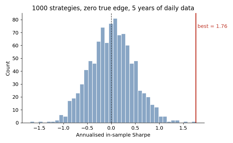
Take N candidate strategies. Give every one of them zero true edge: daily returns drawn i.i.d. from \mathcal{N}(0, \sigma^2) with mean exactly zero. Nothing here can predict anything. Now compute each strategy’s annualised in-sample Sharpe and keep the best — exactly what a naive strategy search does.
import numpy as np

RNG = np.random.default_rng(42)
A, T = 252, 1260          # 252 trading days/yr; T = 5 years of daily data

def ann_sharpe(returns):  # returns shape (T, N) -> (N,)
    mu = returns.mean(axis=0)
    sd = returns.std(axis=0, ddof=1)
    return np.sqrt(A) * mu / sd

N = 1000
sr = ann_sharpe(RNG.standard_normal((T, N)))   # every strategy has TRUE Sharpe 0
print(sr.mean(), sr.max())   # ~0.01,  1.76
The average strategy sits at a Sharpe of ~0, as it should. But the best of the thousand posts an annualised Sharpe of 1.76 over a five-year backtest — the kind of number that gets a strategy funded — purely from sampling noise.
Why it scales like √(2 ln N)
There’s a clean way to see how bad this gets. Under the null of zero edge, the estimated Sharpe over T i.i.d. observations is approximately normal,
\widehat{SR} \;\sim\; \mathcal{N}\!\left(0,\; \tfrac{1}{T}\right) \quad\text{(per-period)},\qquad \widehat{SR}_{\text{ann}} \;\sim\; \mathcal{N}\!\left(0,\; \tfrac{A}{T}\right),
so the standard error of an annualised Sharpe is \sqrt{A/T}. For T=1260 that is \sqrt{252/1260}\approx 0.45 — already a wide band around zero.
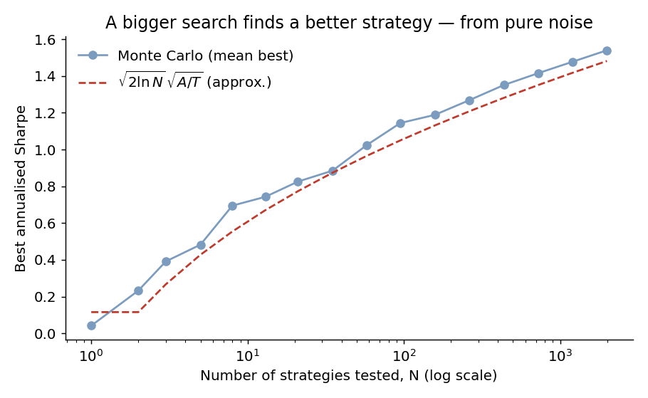
Now the punchline. The expected maximum of N i.i.d. standard normals grows like \sqrt{2\ln N}. Mapping back to annualised Sharpe units, the best spurious Sharpe from N independent trials scales as
\mathbb{E}\!\left[\max_{i\le N}\widehat{SR}_{\text{ann}}^{(i)}\right] \;\approx\; \sqrt{\tfrac{A}{T}}\;\sqrt{2\ln N}.
It grows without bound in N — slowly, but relentlessly. Simulating the mean best Sharpe across many draws tracks this curve closely:
Put in a table, the expected best Sharpe from zero-edge strategies over five years of daily data is:
| Strategies tested N | Expected best annualised Sharpe |
|---|---|
| 10 | ~0.6 |
| 100 | ~1.1 |
| 1,000 | ~1.4 |
| 10,000 | ~1.7 |
A grad student trying a few hundred feature combinations is already in Sharpe-1 territory before adding a single unit of real signal.
The correction: the Deflated Sharpe Ratio
The fix is not to distrust all backtests — it’s to judge an observed Sharpe against the distribution of the best you’d expect under the null, given how many things you tried. Bailey and López de Prado formalise this as the Deflated Sharpe Ratio (DSR). The key input is the expected maximum Sharpe across N trials,
\mathbb{E}\!\left[\max_n SR\right] \approx \sqrt{\operatorname{Var}(SR_n)}\, \Big[(1-\gamma)\,\Phi^{-1}\!\left(1-\tfrac1N\right) + \gamma\,\Phi^{-1}\!\left(1-\tfrac1{N e}\right)\Big],
where \gamma\approx 0.5772 is the Euler–Mascheroni constant, \Phi^{-1} is the inverse normal CDF, and \operatorname{Var}(SR_n) is the variance of Sharpe estimates across the trials you ran. The DSR then asks how far your observed Sharpe sits above this benchmark, correcting for sample length, and for the skew and kurtosis of the strategy’s returns (both of which make extreme Sharpes more likely than the normal approximation suggests). My \sqrt{2\ln N} expression above is just the leading-order version of the bracket.
In practice the corrections that matter are mundane:
- Count your trials honestly. Every feature, parameter, and universe you tried is a trial — including the ones you discarded. The effective N is almost always larger than you think.
- Hold out data you never touch, and treat a strategy as unproven until it survives a clean out-of-sample window.
- Prefer fewer, hypothesis-driven tests to brute-force search. Lower N is the cheapest variance reduction available.
- Report the deflated number, not the cherry-picked one.
Limitations of this demonstration
This is a deliberately clean caricature, and it overstates realism in two directions. The trials here are independent; real candidate strategies are highly correlated, so the effective number of independent trials is smaller than the raw count — the honest N for the DSR is nearer the number of independent bets. Conversely, real return series have fat tails and serial dependence, which the i.i.d. normal draw ignores and which push extreme Sharpes higher than shown. The \sqrt{2\ln N} result is also asymptotic; at small N the finite-sample expected maximum sits a little below it. None of this changes the qualitative conclusion — it only shifts where the curve sits.
References
- Bailey, D. H., & López de Prado, M. (2014). The Deflated Sharpe Ratio: Correcting for Selection Bias, Backtest Overfitting, and Non-Normality. Journal of Portfolio Management, 40(5).
- Bailey, D. H., Borwein, J., López de Prado, M., & Zhu, Q. J. (2017). The Probability of Backtest Overfitting. Journal of Computational Finance, 20(4).
- Harvey, C. R., & Liu, Y. (2015). Backtesting. Journal of Portfolio Management, 42(1).
- Harvey, C. R., Liu, Y., & Zhu, H. (2016). … and the Cross-Section of Expected Returns. Review of Financial Studies, 29(1).
Full script: code/backtest_overfitting.py. Reproduce the figures with python code/backtest_overfitting.py.