Covariance & Correlation
Do two return series move together — and the normalised number that makes it comparable
Variance describes one asset. Covariance and correlation describe how two assets move together — the statistic diversification is built on. Covariance gives the direction and raw size of the co-movement; correlation rescales it into a pure number between −1 and +1 that you can compare across any pair.
The equation
\sigma_{XY} \;=\; \frac{1}{n-1}\sum_{t=1}^{n}\left(r_{X,t}-\bar r_X\right)\left(r_{Y,t}-\bar r_Y\right) \qquad \rho_{XY} \;=\; \frac{\sigma_{XY}}{\sigma_X\,\sigma_Y}
Covariance averages the product of the two assets’ deviations from their means: positive when they tend to move the same way, negative when they offset. Correlation divides that by the two standard deviations, giving a unitless number in [-1, 1].
What each symbol means
| Symbol | Meaning |
|---|---|
| \sigma_{XY} | the sample covariance of returns X and Y (in return²) |
| \rho_{XY} | the correlation of X and Y — unitless, in [-1,1] |
| r_{X,t},\, r_{Y,t} | the period-t returns of X and Y (simple returns) |
| \bar r_X,\, \bar r_Y | their sample means |
| \sigma_X,\, \sigma_Y | their standard deviations |
| n | the number of paired observations |
Covariance is variance’s two-asset generalisation: set Y = X and it collapses to \sigma_{XX} = \sigma_X^2.
Plain-English explanation
For each period, ask whether the two assets were both above their means together, or one up while the other was down. Covariance multiplies the two deviations and averages them: it comes out positive when they tend to move the same way, negative when they offset. But covariance is in “return²” and its size rides on each asset’s volatility, so the raw number is hard to read.
Correlation fixes that. Divide covariance by the two standard deviations and you get a pure number: +1 is lockstep, -1 is mirror images, 0 is no linear relationship. Covariance tells you the direction; correlation makes the strength comparable across every pair.
Why it matters in markets
Covariance is the engine of diversification. A portfolio’s variance is not the average of its parts — it is \mathbf{w}^\top \Sigma\, \mathbf{w}, where \Sigma is the covariance matrix, so the off-diagonal covariances decide how much risk cancels out. Two assets at \rho = 1 give no risk reduction; at \rho = -1 you can hedge risk away entirely; everything useful happens in between. Correlation is the input to pairs trading, hedge ratios, factor models, and mean–variance optimisation.
Like variance, covariance scales with time — multiply by 252 to annualise. Correlation is scale-free: annualising, or switching returns from percent to basis points, leaves \rho unchanged. That invariance is exactly why we quote correlation rather than covariance.
A simple worked example
Two assets over three periods — X = [+2\%, -1\%, +3\%] (mean 1.33\%) and Y = [+1\%, 0\%, +2\%] (mean 1\%):
\sigma_{XY} = \frac{(0.0067)(0) + (-0.0233)(-0.01) + (0.0167)(0.01)}{3-1} = \frac{0.0004}{2} = 0.0002.
With \sigma_X = 2.08\% and \sigma_Y = 1.00\%,
\rho_{XY} = \frac{0.0002}{0.0208 \times 0.0100} = 0.96.
The covariance alone, 0.0002, is unreadable; the correlation, 0.96, tells you immediately these two move almost in lockstep.
Python implementation
import numpy as np
import pandas as pd

X = np.array([0.02, -0.01, 0.03])
Y = np.array([0.01,  0.00, 0.02])

# --- covariance and correlation, spelled out to match the formula ------------
xd, yd = X - X.mean(), Y - Y.mean()             # each asset's deviations from its mean
cov  = (xd * yd).sum() / (len(X) - 1)           # sample covariance (divide by n-1)
corr = cov / (X.std(ddof=1) * Y.std(ddof=1))    # normalise by the two std devs
print(round(cov, 6), round(corr, 4))            # -> 0.0002   0.9608

# --- the whole matrix at once (what you actually use) -----------------------
df = pd.DataFrame({"X": X, "Y": Y})
print(df.cov())     # covariance matrix   (diagonal = each asset's variance)
print(df.corr())    # correlation matrix  (diagonal = 1)
A useful consistency note: unlike std, both numpy.cov and pandas.cov default to the sample divisor (n-1), and corrcoef / corr are scale-free — so the ddof trap from Variance doesn’t bite here.
Manual / Excel calculation
By hand: (1) each asset’s mean, (2) each period’s deviations, (3) multiply the paired deviations, (4) sum, (5) ÷ (n-1) → covariance, (6) ÷ (\sigma_X\sigma_Y) → correlation.
In Excel, with X in B2:B4 and Y in C2:C4:
| Task | Formula |
|---|---|
| Sample covariance | =COVARIANCE.S(B2:B4, C2:C4) → 0.0002 |
| Correlation | =CORREL(B2:B4, C2:C4) → 0.96 |
| Population covariance | =COVARIANCE.P(B2:B4, C2:C4) (÷ n) |
CORREL needs no sample-vs-population choice — being scale-free, it gives the same answer either way.
Financial-market example — Nasdaq 100
The same window — daily returns of AAPL, MSFT, NVDA, PEP and the ^NDX index, 1 Jul 2025 to 30 Jun 2026, n = 251.
import pandas as pd

r = (pd.read_csv("../multi_daily.csv", index_col="Date", parse_dates=True)
       .pct_change().loc["2025-07-01":"2026-06-30"])

print(round(r["AAPL"].cov(r["MSFT"]), 8))    # -> 0.00004367   covariance (return^2)
print(round(r["AAPL"].corr(r["MSFT"]), 4))   # -> 0.1720       correlation
print(r[["NDX","AAPL","MSFT","NVDA","PEP"]].corr().round(2))   # the full matrix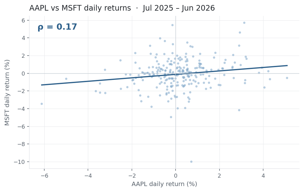
Two things stand out, and both are the whole point of this entry. First, AAPL and MSFT correlate only 0.17 over the year — far below the “big tech all moves together” intuition. Correlation is empirical: you measure it, you don’t assume it. Second, the rest of the matrix:
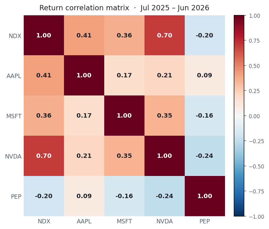
NVDA tracks the index at 0.70 — it is one of the largest weights, so it partly is the index — while PEP, a consumer-staples name, is negatively correlated with the tech complex (−0.16 to −0.24). That negative cell is diversification made visible: adding PEP to a tech book removes risk in a way that adding another chip name never could.
Data from multi_pull.py (yfinance, adjusted closes) in multi_daily.csv. Code blocks are illustrative — the site doesn’t execute them, so every figure was computed and checked against that file.
Common mistakes
- Correlation is not causation. A high \rho says two series moved together over a window, nothing about why, or whether it lasts.
- It only measures linear association. Two series can be tightly related (e.g. one tracks the other’s magnitude) yet show \rho \approx 0. A scatter plot catches what a single number hides.
- Correlations aren’t stable. They drift with regime and tend to spike toward +1 in a crash — right when diversification is supposed to help. A calm-period \rho understates crisis co-movement.
- Reading covariance’s magnitude. It is scale-dependent and in return²; only correlation is comparable across pairs. Use covariance for portfolio maths, correlation for interpretation.
- Covariance/correlation of prices, not returns. Two trending price series look spuriously, near-perfectly correlated. Always use returns.
- Misaligned or too-short samples. Different holiday calendars silently misalign pairs — align on dates first — and a few weeks of data give a \rho that is mostly noise.