Entropy

The average surprise in a distribution — the unit of uncertainty behind cross-entropy and decision trees

Shannon entropy H = −Σ p log p: the average surprise, or uncertainty, in a distribution. Bits vs nats, why it maxes at uniform, the link to cross-entropy and information gain, and the Nasdaq’s near-maximal daily uncertainty.

The cross-entropy entry kept running into a floor: no matter how you scored the Nasdaq’s up/down labels, you couldn’t push the log loss below a certain number — and that number, 0.686 nats, was the entropy of the labels. Entropy is the quantity underneath: the average surprise, or uncertainty, in a probability distribution. It sets the floor for any forecast, defines what “information” means in machine learning, and is the yardstick decision trees use to choose where to split. Claude Shannon defined it in 1948, and it has run through information theory ever since.

The equation

The entropy of a distribution with probabilities p_1, \dots, p_K:

H = -\sum_{i=1}^{K} p_i \log p_i

Using \log_2 gives entropy in bits; the natural log gives nats. The surprise of a single outcome is -\log(p_i); entropy is the average surprise, weighted by how often each outcome occurs.

What each symbol means

Symbol	Meaning
H	the entropy — uncertainty of the distribution
p_i	probability of outcome i
K	the number of possible outcomes
-\log(p_i)	the surprise (information content) of outcome i
\log	\log_2 (bits) or \ln (nats)

Plain-English explanation

Entropy measures how uncertain a distribution is — equivalently, how surprised you expect to be by its outcome. A rare event carries a lot of surprise (a one-in-a-million outcome is astonishing when it lands, -\log_2(10^{-6}) \approx 20 bits); a near-certain event carries almost none. Entropy averages that surprise over all outcomes, weighting each by its probability. The result is largest when the distribution is uniform — every outcome equally likely, nothing to predict — and smallest (zero) when one outcome is certain, because then there is no surprise at all.

For a coin, entropy traces the inverted-U in the figure: a fair coin (0.5) sits at the maximum, 1 bit, because it is maximally unpredictable; a bent coin that lands heads 90% of the time has only 0.47 bits, because you can usually guess right; a two-headed coin has zero. In general, K equally-likely outcomes have entropy \log_2(K) bits — 1 bit for a coin, 2.58 for a die — which is the maximum any K-outcome distribution can have, and also exactly the number of yes/no questions you’d need to pin down the outcome. That “bits to encode” reading is Shannon’s: entropy is the shortest average description length of a random source.

Why it matters in markets

Entropy is the bridge between the two halves of this section — it is the same quantity the classification losses were minimising, now named. Minimising cross-entropy drives the model’s predicted distribution toward the true one, and cross-entropy decomposes exactly as entropy plus a penalty for being wrong (the KL divergence): H(y, p) = H(y) + \text{KL}(y\,\|\,p). Because that penalty can’t be negative, cross-entropy can never fall below the entropy of the labels — that is the floor the previous entry hit. The entropy of the data is the irreducible uncertainty; a model earns its keep only by the amount it shaves cross-entropy below that floor.

Entropy is also the engine of decision trees. A tree decides where to split by asking which question most reduces uncertainty — and “uncertainty” here is entropy. The drop in entropy from a split is the information gain (the next entry); the Gini impurity that follows is a close cousin. So the same idea that grades a neural network’s probabilities also grows a random forest. And in markets it gives a clean way to say how predictable something is: the entropy of the Nasdaq’s daily direction, as the figure shows, is 0.99 of the maximum 1 bit — the market is telling you, in the native units of information, that its next move is very nearly a coin flip.

A simple worked example

Compare three sources. A fair coin has two equally-likely outcomes, so H = -(0.5\log_2 0.5 + 0.5\log_2 0.5) = 1 bit. A fair die has six, all at 1/6, so H = \log_2(6) = 2.58 bits — more outcomes, more uncertainty. A biased coin landing heads 90% of the time has H = -(0.9\log_2 0.9 + 0.1\log_2 0.1) = 0.47 bits — fewer effective outcomes, less uncertainty, because you can usually guess heads. Entropy rises with the number of possibilities and falls as the distribution tilts toward one of them.

Python implementation

import numpy as np

def entropy(p, base=2):                     # base 2 -> bits, np.e -> nats
    p = np.asarray(p, float)
    p = p[p > 0]                            # 0*log0 := 0
    return -(p * (np.log(p) / np.log(base))).sum()

entropy([0.5, 0.5])                         # -> 1.0 bit   (fair coin)
entropy([0.56, 0.44])                       # -> 0.990 bits (NDX daily up/down)

scipy.stats.entropy does this (default base e). Note 0 \cdot \log 0 is defined as 0, so zero-probability outcomes are simply dropped.

Manual / Excel calculation

Per outcome, compute =-p*LOG(p,2) (bits) and sum the column, or in one cell =SUMPRODUCT(-probs, LOG(probs,2)). Use LN in place of LOG(...,2) for nats. Guard against empty cells — a probability of 0 must contribute 0, not an error.

Financial-market example — Nasdaq 100

Ask the information-theoretic version of “is the Nasdaq predictable?” The daily up/down label is up 56% of the time, so its entropy is H(0.56) = 0.990 bits — 99% of the one-bit maximum a binary outcome can carry. Knowing nothing, the market’s next daily move is worth almost a full bit of surprise: it is nearly a fair coin. This is the same 0.686 nats that was the floor on cross-entropy in the last entry — entropy and that log-loss floor are literally the same number in different units.

Left: binary entropy peaks at 1 bit for a 50/50 split; NDX daily up/down (0.56) sits at 0.99 bits, a predictable 0.90 event at 0.47. Right: bits of uncertainty in a direction call — fair coin 1.00, NDX daily 0.99, NDX monthly 0.945, a genuine 0.70 edge 0.881.

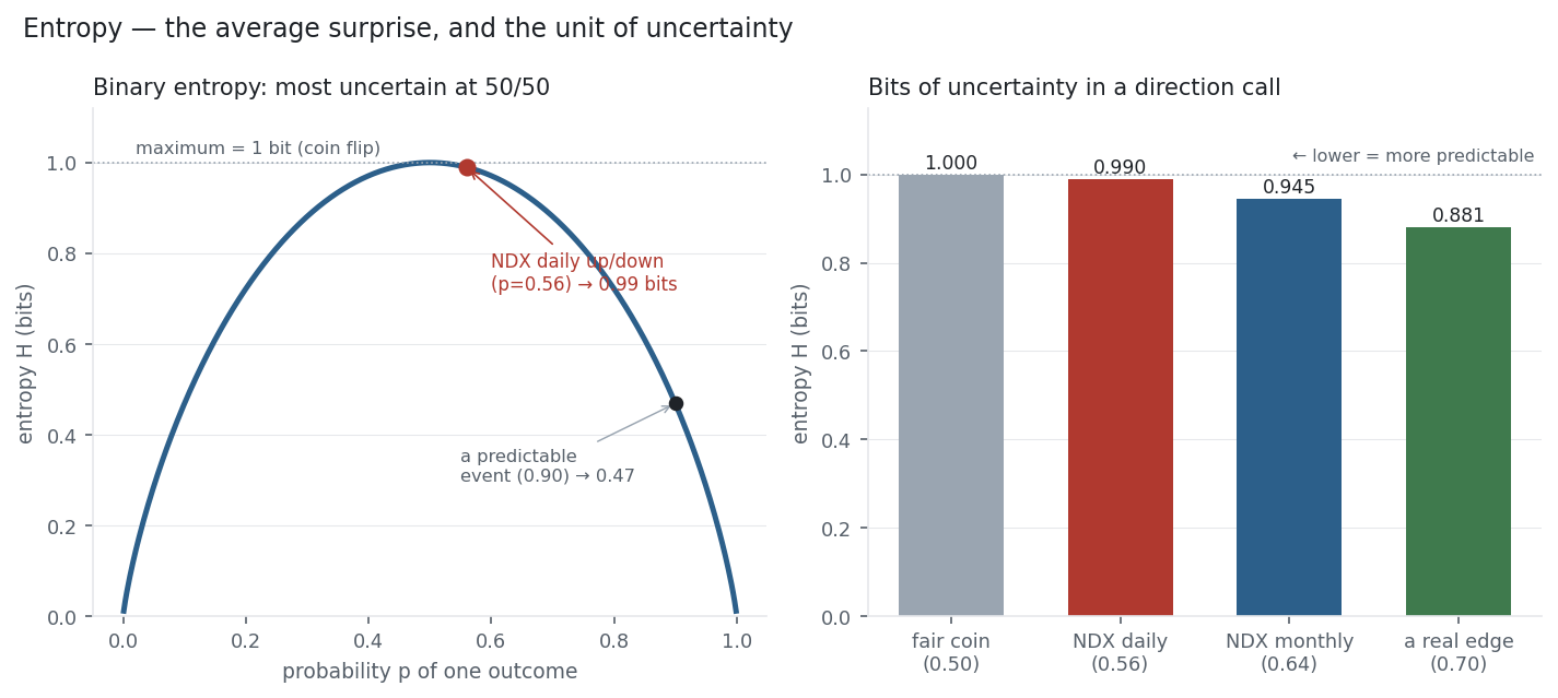
Two contrasts sharpen it. Split tomorrow’s return into three equal-sized regimes and the entropy is 1.585 bits — exactly \log_2(3), the maximum for three outcomes — so a typical day’s regime is as uncertain as it could possibly be. But zoom out to monthly direction, up 64% of the time, and entropy falls to 0.945 bits: the upward drift accumulates over a month, so the direction of a longer horizon is modestly more predictable than a single day’s, even though neither is tradable on its own. Entropy quantifies exactly how much — and how little — the market gives away.

Same multi_daily.csv as the previous entries (yfinance, adjusted closes). Entropies are of the empirical up/down (and 3-class tercile) label distributions; the daily figure equals the base-rate cross-entropy of the previous entry (0.686 nats = 0.990 bits). Every number was checked.

Common mistakes

• Forgetting the base. Bits (\log_2) and nats (\ln) differ by a factor of \ln 2 \approx 0.693; state which you’re using and don’t mix them.
• Mishandling zero probabilities. 0 \cdot \log 0 is defined as 0, not undefined; drop zero-probability outcomes rather than erroring.
• Confusing entropy with variance. Both measure spread, but entropy depends only on the probabilities, not the outcome values — a distribution over \{1, 2\} and over \{1, 1000\} with the same probabilities has the same entropy.
• Reading high entropy as “bad”. High entropy just means high uncertainty; for a genuinely random process that is correct, not a flaw.
• Assuming a maximum of 1. One bit is the max only for two outcomes; K outcomes cap at \log_2(K).
• Treating it as directional. Entropy is about uncertainty, not which way; a 56/44 and a 44/56 split have identical entropy.