GARCH
Modelling the volatility, not the mean — why calm follows calm and storms follow storms
Every model so far has chased the mean of returns — and found almost nothing, because returns are close to unpredictable. GARCH changes the target. It gives up on forecasting the return and forecasts its volatility instead, and there the news is much better: volatility is highly predictable. The autocorrelation entry already showed why — squared returns have a large, slowly-decaying ACF (calm clusters with calm, turbulence with turbulence). GARCH is the model built to capture exactly that clustering, and it is the volatility engine that bolts onto the ARIMA mean this section just built.
The equation
A return is a mean plus a shock whose size changes over time; GARCH(1,1) is the recursion for that size:
r_t = \mu + \varepsilon_t, \quad \varepsilon_t = \sigma_t z_t, \quad z_t \sim \mathcal{N}(0,1)
\sigma_t^2 = \omega + \alpha\,\varepsilon_{t-1}^2 + \beta\,\sigma_{t-1}^2
Today’s variance is a baseline \omega, plus a reaction to yesterday’s squared shock (\alpha), plus a memory of yesterday’s variance (\beta).
What each symbol means
| Symbol | Meaning |
|---|---|
| r_t | the return at time t |
| \mu | the (small, near-constant) mean return |
| \varepsilon_t | the shock / residual — return minus mean |
| \sigma_t^2 | the conditional variance at time t — what GARCH forecasts |
| z_t | a standardised random draw (mean 0, variance 1) |
| \omega | omega — the constant / baseline variance |
| \alpha | alpha — reaction to the latest shock (the ARCH term) |
| \beta | beta — persistence of past variance (the GARCH term) |
\alpha + \beta is the persistence of volatility; it must be < 1 for a finite long-run variance \omega/(1-\alpha-\beta).
Plain-English explanation
GARCH stands for Generalized AutoRegressive Conditional Heteroskedasticity — a mouthful that just means “a model where the variance changes over time and depends on its own past.” Ordinary models assume a return’s shock has a fixed size (constant variance, “homoskedastic”). GARCH lets that size breathe: after a big move, the next day’s expected volatility rises; after a run of calm, it falls. The recursion \sigma_t^2 = \omega + \alpha\varepsilon_{t-1}^2 + \beta\sigma_{t-1}^2 says today’s variance is a blend of three things — a long-run baseline (\omega), how violent yesterday actually was (\alpha times yesterday’s squared shock), and how volatile the model already thought things were (\beta times yesterday’s variance).
The two coefficients split the labour. \alpha is the reaction — how sharply volatility jumps when a shock lands. \beta is the persistence — how long a raised volatility lingers. Their sum, \alpha + \beta, is the memory of volatility: the closer to 1, the more slowly a spike decays. For equity indices it is typically around 0.95–0.99, so volatility shocks fade over weeks, not days — which is exactly the clustering you see on any price chart.
Why it matters in markets
GARCH matters because volatility, unlike return, is forecastable — and volatility is what risk is made of. A single standard deviation assumes one fixed volatility for all time; GARCH replaces it with a volatility that updates every day, which transforms three things. Risk measures: Value at Risk and Expected Shortfall computed on a GARCH volatility rise and fall with the market instead of lagging it, so limits tighten going into turbulence rather than after it. Fat tails: because the variance itself varies, GARCH manufactures the excess kurtosis of real returns even when the shocks z_t are perfectly normal — a mixture of normals with different variances is fat-tailed. And option pricing and position sizing both live or die on a volatility forecast.
It also completes this section’s division of labour. ARIMA models the conditional mean and assumes constant-variance shocks; GARCH models the conditional variance of exactly those shocks. Run together (an ARIMA-GARCH), one engine forecasts where the series is heading and the other how uncertain that forecast is — and for a near-efficient market, the honest finding of the last few entries is that the second engine is the one doing all the useful work.
A simple worked example
Take GARCH(1,1) with \omega = 0.02, \alpha = 0.10, \beta = 0.88 (variance in %² per day). Yesterday delivered a −3% shock while the model’s variance stood at \sigma^2 = 1.2^2 = 1.44. Today’s variance is:
\sigma_t^2 = 0.02 + 0.10\times(-3)^2 + 0.88\times1.44 = 0.02 + 0.90 + 1.27 = 2.19,
so \sigma_t = \sqrt{2.19} \approx 1.48\% per day. The 3% shock lifted tomorrow’s expected volatility from 1.2% to 1.48%. Left alone it decays back toward the long-run level \sigma = \sqrt{\omega/(1-\alpha-\beta)} = \sqrt{0.02/0.02} = 1.0\%/day, with a half-life of \ln(0.5)/\ln(0.98) \approx 34 days. Big day today, jumpy tomorrow, slowly calming after — the arithmetic of clustering.
Python implementation
from arch import arch_model
import pandas as pd

r = (pd.read_csv("../multi_daily.csv", index_col="Date", parse_dates=True)["NDX"]
       .pct_change().dropna() * 100)             # percent returns (arch prefers scaled)

res = arch_model(r, mean="Constant", vol="GARCH", p=1, q=1).fit(disp="off")
a, b = res.params["alpha[1]"], res.params["beta[1]"]
print(round(a, 3), round(b, 3), round(a + b, 3))    # -> 0.132 0.843 0.975
cond_vol = res.conditional_volatility * (252 ** 0.5)  # annualised volatility series
The arch package is the standard; p is the ARCH order, q the GARCH order. Scale returns by 100 for the optimiser, and remember the fitted variance is in those squared units.
Manual / Excel calculation
GARCH fitting needs maximum likelihood, but the recursion is a one-cell spreadsheet formula once you have \omega, \alpha, \beta: =omega + alpha*E1^2 + beta*F1, where E is the shock column and F the previous variance. Seed the first variance with the sample variance and fill down — you’ll reproduce the conditional-variance path exactly. Estimating the three parameters by hand isn’t practical; use the arch package or R’s rugarch.
Financial-market example — Nasdaq 100
Fit GARCH(1,1) to eleven years of NDX daily returns and it puts hard numbers on volatility clustering: \alpha = 0.13 (a meaningful jump in variance the day after a shock) and \beta = 0.84 (most of yesterday’s volatility carries into today), for a persistence of \alpha + \beta = 0.975. That near-1 sum is the whole story — a volatility spike decays with a half-life of about 27 days, so a turbulent week echoes for a month. The model’s long-run volatility works out to 23%/yr, essentially the 22% sample figure, confirming it is well specified.
| GARCH(1,1) on NDX | value | meaning |
|---|---|---|
| \alpha (reaction) | 0.13 | variance jump after a shock |
| \beta (persistence) | 0.84 | yesterday’s variance carried over |
| \alpha + \beta | 0.975 | slow decay — vol half-life ≈ 27 days |
| long-run vol | 23%/yr | matches the 22% sample vol |
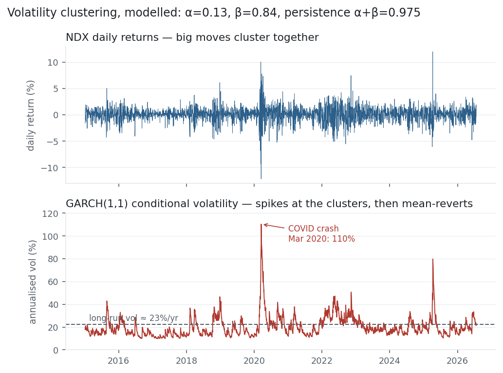
The figure makes the fit visible. NDX returns obviously cluster — a violent 2020, a jumpy 2022, calm stretches between — and the GARCH conditional volatility tracks it exactly, spiking to 110%/yr in the March 2020 crash and sinking below 10% in quiet spells, always pulled back toward the 23% long-run line. This is the predictability the mean models never had: you can’t say whether tomorrow is up or down, but you can say, with real skill, whether it will be calm or wild. The squared-return autocorrelation of 0.39 that the autocorrelation entry flagged is precisely what GARCH monetises.
Same multi_daily.csv as the previous entries (yfinance, adjusted closes); GARCH(1,1) with normal innovations via the arch package. A Student-t fit tightens the tails but pushes persistence to 0.997 (near-IGARCH) — normal is the cleaner baseline here. Every number was computed and checked.
Common mistakes
- Modelling the mean with GARCH. GARCH forecasts variance, not direction; it says nothing about whether returns go up or down.
- Forgetting \alpha + \beta < 1. If the sum hits 1 the long-run variance is undefined (IGARCH); a Student-t fit here drifts to 0.997, where “long-run vol” becomes meaningless — check it.
- Using raw (unscaled) returns. The optimiser struggles with tiny numbers; scale returns ×100 and track the variance units.
- Assuming normal shocks are enough. GARCH with normal z fattens the tails, but real returns are fatter still — a Student-t often fits better (at the cost of higher persistence).
- Ignoring asymmetry. Volatility rises more after down moves than up (the leverage effect); plain GARCH is symmetric — use GJR-GARCH or EGARCH if that matters.
- Reading conditional vol as a tradable return. Predicting volatility is not predicting return; you trade it through options or position sizing, not by forecasting direction.