Information Gain

How much a split cuts uncertainty — the rule a decision tree uses to choose its questions

Information gain = parent entropy − weighted child entropy: the uncertainty a split removes. Why decision trees maximise it, its identity with mutual information, the high-cardinality bias, and a near-zero Nasdaq split.

Entropy measured how uncertain a distribution is; information gain measures how much a question reduces that uncertainty. Ask “was today an up day?” and split your data into the up-days and the down-days: if the two groups have more predictable labels than the whole, you’ve gained information. Information gain is exactly that reduction in entropy — and it is the criterion a decision tree uses to choose, at every node, which question to ask. It is also, under another name, the mutual information between a feature and the label.

The equation

For a set S split by a feature into subsets S_v:

\text{IG}(S, \text{split}) = H(S) - \sum_{v} \frac{|S_v|}{|S|}\, H(S_v)

The entropy of the parent minus the weighted average entropy of the children — the uncertainty the split removes.

What each symbol means

Symbol	Meaning
IG	information gain (bits or nats)
H(S)	entropy of the parent set
S_v	the subset (child) for split value v
|S_v|/|S|	fraction of samples landing in child v
H(S_v)	entropy of child v

Plain-English explanation

A decision tree grows by asking questions that carve the data into purer groups. Information gain scores each candidate question by how much purer the groups become. Start with the parent’s entropy — the uncertainty in its labels. Apply a split, and each child has its own entropy; average those, weighted by how many samples land in each child. The drop from parent entropy to that weighted-child entropy is the information gain: the bits of uncertainty the question removed. A question that perfectly separates the classes drives the children to zero entropy and gains the full parent entropy; a useless question leaves the children as mixed as the parent and gains nothing.

The name is literal. Because entropy is expected surprise, a split that lowers it has told you something — and the amount is exactly the mutual information between the feature and the label, I(\text{feature}; \text{label}): how many bits knowing the feature reveals about the answer. It is always non-negative (a split can’t, in expectation, make you more uncertain), which is why greedily maximising it — pick the highest-gain question, recurse on each child — is a sensible way to grow a tree. The one catch is that raw information gain favours features with many distinct values (an ID column splits every sample into its own zero-entropy child and “gains” everything while learning nothing), which is why C4.5 divides by the split’s own entropy to get the gain ratio.

Why it matters in markets

Information gain is how tree-based models — decision trees, and the random forests and gradient-boosted machines built from them — decide what to look at, so it is doing the feature selection inside some of the most-used models in quant finance. A feature earns a place near the top of a tree only if splitting on it removes real uncertainty about the target; information gain is the referee. That makes it, like entropy and cross-entropy before it, a clean detector of genuine signal: if no split on a feature gains meaningful information, the feature is noise for that target, and a tree will correctly ignore it.

On markets that referee is unforgiving. Splitting tomorrow’s up/down label on today’s return — the natural first question a tree would try — gains almost nothing, because the two children (up-days-after and down-days-after) are barely less mixed than the whole. The tiny gain is the same faint mean reversion the whole library keeps measuring, now in the currency of information: real, but a rounding error against the day’s near-full bit of uncertainty. A tree fed only today’s return to predict tomorrow’s direction would find nothing worth splitting on — the honest, and correct, outcome.

A simple worked example

Ten samples, 5 up and 5 down, so the parent entropy is H(5/5) = 1 bit. Try a split that sends most ups one way: the left child gets 4 up and 1 down, the right gets 1 up and 4 down. Each child has entropy H(0.8) = 0.72 bits, and since each holds half the data the weighted child entropy is 0.72. The information gain is 1 - 0.72 = 0.28 bits — the split removed a bit more than a quarter of the uncertainty. A perfect split (5 up on one side, 5 down on the other) would drive both children to zero entropy and gain the full 1 bit; a useless split (still 50/50 in each child) would gain 0.

Python implementation

import numpy as np

def entropy(y):
    _, c = np.unique(y, return_counts=True); p = c / c.sum()
    return -(p * np.log2(p)).sum()

def information_gain(y, mask):                     # mask picks the left child
    n = len(y); yl, yr = y[mask], y[~mask]
    child = len(yl)/n*entropy(yl) + len(yr)/n*entropy(yr)
    return entropy(y) - child

# a tree tries every feature/threshold and keeps the split with the largest gain

sklearn’s DecisionTreeClassifier(criterion="entropy") maximises exactly this at each node; criterion="gini" (the next entry) is the usual faster default.

Manual / Excel calculation

For a binary split: compute the parent entropy =-p*LOG(p,2)-(1-p)*LOG(1-p,2), then the same for each child, then IG = H_parent - (n_left/n)*H_left - (n_right/n)*H_right. Trying a handful of thresholds by hand and keeping the biggest IG is exactly (if slowly) what a tree does.

Financial-market example — Nasdaq 100

Put a decision tree’s first question to the Nasdaq: to predict whether tomorrow is an up day, what’s the best split on today’s return? The parent entropy is 0.99 bits (from the entropy entry — the market’s near-maximal daily uncertainty). Scanning every threshold, the best split — today’s return below about 1.25% versus above — reduces that by 0.0008 bits, or 0.77 milli-bits: eight hundredths of one percent of the uncertainty.

Left: a decision-tree split — parent (5↑5↓, H=1.00 bit) into children (4↑1↓ and 1↑4↓, H=0.72 each), gaining 0.28 bits. Right: information gain vs split threshold on NDX today’s return — across every threshold it never clears a single milli-bit (best ≈ 0.77 milli-bits, 0.08% of the uncertainty).

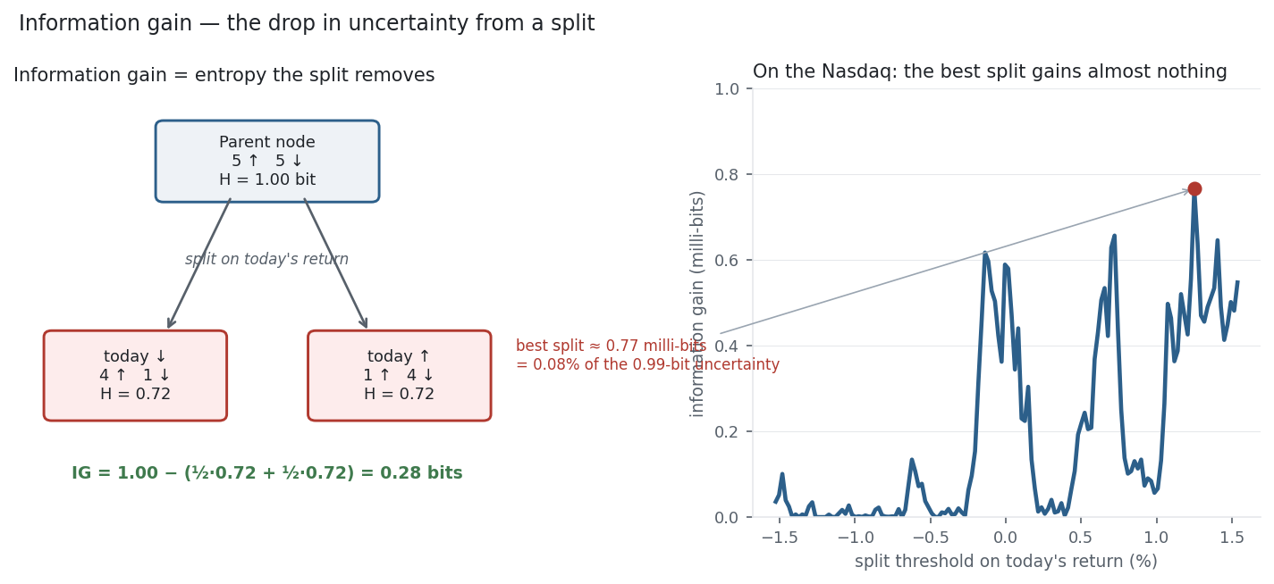
The left panel shows what a useful split looks like — a feature that cleaves 5-up-5-down into 4/1 and 1/4 gains 0.28 bits. The right panel shows the reality: across every threshold on today’s return, the information gain never clears a single milli-bit. A tree offered only today’s return to forecast tomorrow’s direction would shrug — no question it can ask meaningfully lowers the uncertainty. That near-zero gain is not a flaw in the method; it is the method correctly reporting that today’s move tells you almost nothing about tomorrow’s — the same verdict autocorrelation, cross-entropy, and entropy each delivered in their own units.

Same multi_daily.csv as the previous entries (yfinance, adjusted closes). The parent is tomorrow’s NDX up/down label (entropy 0.99 bits); information gain is scanned over thresholds on today’s return, requiring each child to keep ≥ 50 samples. Every number was checked.

Common mistakes

• Favouring high-cardinality features. Raw information gain is inflated by features with many distinct values; use the gain ratio (gain ÷ split entropy), or Gini, to counter it.
• Reading gain as importance out of context. A split’s gain depends on its parent; the same feature can gain a lot high in a tree and nothing lower down.
• Forgetting to weight the children. Information gain uses the sample-weighted average of child entropies, not the plain average — a tiny child counts little.
• Confusing it with accuracy. A split can raise information gain without changing majority-vote accuracy; the two optimise different things.
• Chasing gain on the training set. High in-sample gain can be overfitting (the ID-column trap); validate, and prune or limit depth.
• Assuming gain can be negative. In expectation it can’t — a “best” split showing negative gain is a bug (usually an unweighted average).