Mean Return

The first moment of a return series — and why it is not the growth you earned

The arithmetic mean return: estimator of E[r], its gap to compound growth (the volatility drag), and a worked Nasdaq-100 example — by hand, in Python, and in Excel.

The equation

\bar r \;=\; \frac{1}{n}\sum_{t=1}^{n} r_t

The sample arithmetic mean of a return series — the estimator of the first raw moment \mathbb{E}[r]. Sum the per-period returns and divide by their count. Throughout this entry r_t is a simple return, r_t = P_t/P_{t-1} - 1; the arithmetic mean of log returns is a related but distinct object (it annualises additively and equals \ln of the geometric mean of simple returns). The geometric / compound mean — what governs multi-period growth — is deferred to its own entry; here we stay with the arithmetic mean and signpost the difference where it bites.

What each symbol means

Symbol	Meaning
\bar r	the sample mean return — our estimate of \mathbb{E}[r]
r_t	the return in period t, a simple return r_t = P_t/P_{t-1}-1
n	the number of return observations
\sum_{t=1}^{n}	sum over all n observations
\mathbb{E}[r]	the true (population) expected one-period return

\bar r is a statistic computed from a sample; \mathbb{E}[r] is the population parameter it estimates. Keeping the two apart is what the later Core-statistics entries — standard error, t-statistic, confidence interval — are built on.

Plain-English explanation

Add up every period’s return and divide by how many there are. That average is the mean return: the “typical” return per period and the simplest forecast of the next one. Formally it is the first moment of the return distribution — its centre of mass.

Two clarifications that save trouble later. It is an average of returns, not of prices — averaging price levels tells you nothing about performance. And it is arithmetic: a flat average, not the compound rate at which money actually grows (that is the geometric mean, and it is always a little lower).

Why it matters in markets

The mean return is the atom nearly everything else is built from: the numerator of the Sharpe ratio (\bar r - r_f over \sigma), the expected-return term in CAPM, the drift in a return model, and — stacked into a vector — the \mathbf{w}^\top \bar{\mathbf r} that gives a portfolio’s expected return. Under i.i.d. returns it is an unbiased estimate of \mathbb{E}[r], the right quantity for a one-period decision.

What it is not is the growth rate of your capital. Over many periods wealth compounds, and terminal wealth is governed by the geometric mean

g \;=\; \left(\prod_{t=1}^{n}(1+r_t)\right)^{1/n} - 1 \;\approx\; \bar r - \tfrac{1}{2}\sigma^2 .

The arithmetic mean always sits above the geometric mean by roughly half the variance — the volatility drag. So \bar r is the correct input for expected return and risk-adjusted ratios, and the wrong input for what you actually compounded. Confusing the two is the most common error in return maths — which is why this entry leads the library.

A simple worked example

Three periods with returns +2\%, -1\%, +3\%:

\bar r = \frac{0.02 + (-0.01) + 0.03}{3} = \frac{0.04}{3} = 0.0133 = 1.33\%.

The average period return is 1.33%. Compounding the same three returns instead gives 1.02 \times 0.99 \times 1.03 - 1 = 4.01\% total, a geometric mean of 1.32\% per period — already a touch below the arithmetic 1.33\%. With these tiny returns the gap is trivial; with volatile daily returns it is not.

Python implementation

import numpy as np                        # fast vectorised arrays and reductions

# --- the definition, on a tiny return series --------------------------------
r = np.array([0.02, -0.01, 0.03])         # three period returns as decimals (2%, -1%, 3%)
mean_return = r.mean()                     # (1/n) * sum(r_t): the equation in one call
print(mean_return)                         # -> 0.013333333333333334   (1.33%)

# --- spelled out, to match the formula symbol for symbol --------------------
mean_return = r.sum() / r.size             # sum of returns divided by n
print(round(mean_return * 100, 4))         # -> 1.3333   (as a percentage)

# --- from prices: form returns first, THEN average --------------------------
prices  = np.array([100.0, 102.0, 100.98, 104.0094])  # a short price path
returns = prices[1:] / prices[:-1] - 1     # simple return each step: P_t / P_{t-1} - 1
print(returns)                             # -> [ 0.02  -0.01   0.03 ]
print(returns.mean())                      # -> 0.013333...   same mean, from prices

# --- on a real series (pandas), the everyday one-liner ----------------------
import pandas as pd
close = pd.Series(prices)                  # e.g. a column of daily closing prices
mean_daily = close.pct_change().mean()     # pct_change(): P_t/P_{t-1}-1 per row; .mean() skips the leading NaN
print(round(mean_daily * 100, 4))          # -> 1.3333

pct_change() leaves a NaN in the first row (no prior price to divide by); .mean() skips it automatically. A hand-rolled loop must not — divide by the number of returns, not the number of prices.

Manual / Excel calculation

By hand it is one line: sum the returns, divide by the count — 0.02 + (-0.01) + 0.03 = 0.04, then 0.04 / 3 = 0.0133.

In Excel, with the three returns in B2:B4:

Task	Formula
Mean return	=AVERAGE(B2:B4) → 0.0133 (format as %)
The same, spelled out	=SUM(B2:B4)/COUNT(B2:B4)
Returns from prices in A2:A5	=A3/A2-1 in B3, fill down
Mean straight from prices	=AVERAGE(A3:A5/A2:A4-1) (array; Ctrl+Shift+Enter in legacy Excel)
Geometric mean, for contrast	=GEOMEAN(1+B2:B4)-1 (array)

GEOMEAN multiplies the (1+r_t) growth factors and takes the n-th root, so feed it 1+B2:B4, not the raw returns.

Financial-market example — Nasdaq 100

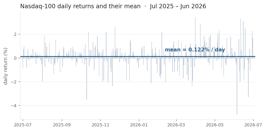
Daily simple returns on the Nasdaq-100 (^NDX) over the twelve months from 1 Jul 2025 to 30 Jun 2026 — n = 251 trading days, the index moving from a base close of 22,679.01 (30 Jun 2025) to 30,276.35 (30 Jun 2026).

Nasdaq-100 daily returns over the window, with the arithmetic mean marked. Most days sit close to the mean; a handful of large moves do most of the pulling.

import pandas as pd

px = pd.read_csv("ndx_daily.csv", parse_dates=["Date"]).set_index("Date")["Close"]
r  = px.pct_change().loc["2025-07-01":"2026-06-30"]   # daily returns, the 1-year window
n  = r.size                                            # 251 trading days

mean_daily = r.mean()                                  # arithmetic mean daily return
ann_arith  = mean_daily * 252                          # annualised by linear scaling (x252)
geo_daily  = (1 + r).prod() ** (1 / n) - 1             # geometric (compound) mean daily return

print(round(mean_daily * 100, 4))   # -> 0.1217   % per day (arithmetic)
print(round(ann_arith  * 100, 2))   # -> 30.68    % annualised (x252)
print(round(geo_daily  * 100, 4))   # -> 0.1152   % per day (geometric)
print(round((px["2026-06-30"] / px["2025-06-30"] - 1) * 100, 2))  # -> 33.50  % actual move

The arithmetic mean daily return is 0.1217%, which annualises (×252) to 30.7% — the expected-return convention, and the number you would feed a Sharpe ratio. The geometric mean is 0.1152% per day, and the index’s actual compound move was +33.50% (a 33.65% CAGR).

The arithmetic mean sits 0.0066 pp/day above the geometric mean, and that gap is almost exactly \tfrac{1}{2}\sigma^2 = 0.0066\% (daily variance) — the volatility drag, made visible. The trap in one line: compounding the arithmetic daily mean over the 251 days, (1.001217)^{251}-1 = +35.7\%, overstates the +33.5% the index actually delivered, while compounding the geometric mean reproduces it to the basis point.

Data pulled with ndx_pull.py (yfinance, ^NDX) into ndx_daily.csv. The site doesn’t execute code, so every figure here was computed and checked against that file rather than rendered live.

Common mistakes

• Treating the mean as growth. Terminal wealth follows the geometric mean, lower by ≈\tfrac{1}{2}\sigma^2. Projecting multi-year growth from the arithmetic mean overstates it — and the more volatile the series, the bigger the overstatement.
• Sloppy annualisation. Multiplying by 252 scales the expected one-period return (right for Sharpe numerators and expected P&L); compounding gives CAGR (right for growth). Different numbers — in the NDX window above they land on opposite sides, 30.7% vs 33.65%, purely because one is linear and one compounds.
• Averaging prices, not returns. The mean of a price series is meaningless for performance. Convert to returns first.
• Mixing simple and log returns. Log returns add across time and annualise cleanly by ×N; simple returns compound. The arithmetic mean of log returns equals the log of the geometric mean of simple returns — so don’t average logs and quote it as a simple mean.
• Trusting a mean from too few points. The standard error of the mean is \sigma/\sqrt{n}, so a great-looking mean over 30 days is mostly noise. Short-sample means are estimates, not facts.
• Forgetting the mean is not robust. One earnings-day gap, or a single unadjusted split in the data, can swing it. Sanity-check for bad ticks and corporate actions first.