The Softmax Function

A vector of scores into a probability distribution — sigmoid for many classes

Softmax: exp-then-normalise a vector of scores into probabilities that sum to 1. Why it reduces to the sigmoid, shift-invariance and numerical stability, temperature, and a 3-class Nasdaq regime example.

Sigmoid turned one score into one probability, for a yes/no question. Softmax does the same job when there are many answers: it takes a vector of scores — one per class — and turns the whole vector into a probability distribution, a set of numbers between 0 and 1 that sum to exactly 1. It is the output layer of every multi-class classifier, from digit recognition to the next-token prediction inside a language model, and it collapses to the sigmoid exactly when there are only two classes.

The equation

For a vector of scores z = (z_1, \dots, z_K), the softmax of the i-th class is:

\text{softmax}(z)_i = \frac{e^{z_i}}{\sum_{j=1}^{K} e^{z_j}}

Each output lies in (0,1) and the K outputs sum to 1 — a probability distribution over the K classes.

What each symbol means

Symbol	Meaning
\text{softmax}(z)_i	probability assigned to class i
z_i	the raw score (logit) for class i
K	the number of classes
e^{z_i}	the exponentiated score (always positive)
\sum_j e^{z_j}	the normaliser (sum over all classes)

Plain-English explanation

Softmax answers “given these scores, how should I split one unit of probability among the classes?” It does it in two moves. First it exponentiates every score — e^z is always positive and grows fast, so this turns arbitrary real numbers into positive weights and stretches the gaps between them (a score two points higher becomes e^2 \approx 7.4\times more weight). Then it normalises — divide each weight by the total — so the results sum to 1 and read as probabilities. Scores of [2, 1, 0.1] become [0.66, 0.24, 0.10]: the biggest score gets the biggest share, but every class keeps some probability.

Two properties are worth holding onto. Softmax is a soft argmax: it picks out the largest score the way argmax does, but smoothly and differentiably, so a model can be trained on it by gradient descent. And it is controlled by a temperature — dividing the scores by T before exponentiating. A high temperature flattens the distribution toward uniform (“I’m not sure”); a low temperature sharpens it toward a single 1 (“I’m certain”); the figure shows the same three scores at three temperatures. With two classes, softmax is exactly the sigmoid — \text{softmax}([z, 0]) has first component \sigma(z) — so everything about the sigmoid is the K = 2 corner of this.

Why it matters in markets

Softmax is the standard way a model expresses a choice among several options as calibrated probabilities, and that framing is often the useful one in markets. Rather than forcing a binary up/down call, you can ask a model to distribute its belief over a set of regimes — down, flat, up; or a set of volatility states; or which of several assets will lead — and softmax gives back a full distribution instead of a single guess, so you can size by conviction and see when the model is genuinely uncertain (a near-uniform output) versus confident (a peaked one).

It is also inseparable from its partner loss. Softmax is almost always trained with cross-entropy (the next entry), because the two together have a beautifully simple gradient: the error signal reduces to just (predicted probability − actual), with the exponential and the normaliser cancelling out. That clean gradient is why softmax-plus-cross-entropy is the default final layer of essentially every classification network. One practical note follows straight from the maths: softmax is unchanged if you add the same constant to every score, so real implementations subtract the largest score first to stop e^z from overflowing — a free trick that prevents NaNs.

A simple worked example

Three classes with scores z = [2, 1, 0.1]. Exponentiate: e^2 = 7.39, e^1 = 2.72, e^{0.1} = 1.11, summing to 11.21. Divide each by the total: [7.39, 2.72, 1.11] / 11.21 = [0.66, 0.24, 0.10], which sums to 1. Class A, two points ahead, takes two-thirds of the probability; class C, the laggard, still keeps 10%. Now sharpen with temperature T = 0.5 (double the scores before exponentiating): the distribution becomes [0.86, 0.12, 0.02] — far more confident in A. The scores’ order never changes; temperature only changes how decisively softmax commits to the leader.

Python implementation

import numpy as np

def softmax(z, T=1.0):
    z = np.asarray(z) / T
    z = z - z.max()                  # shift for numerical stability (result unchanged)
    e = np.exp(z)
    return e / e.sum()

softmax([2, 1, 0.1])                 # -> [0.659, 0.242, 0.099], sums to 1
softmax([1.5, 0])[0]                 # -> 0.8176 == sigmoid(1.5)  (the 2-class case)

The z - z.max() line is not optional in production: without it a large score overflows np.exp to infinity. scipy.special.softmax does this for you.

Manual / Excel calculation

For scores in cells A1:A3: put =EXP(A1) down column B, sum them (=SUM(B1:B3)), then each probability is =B1/SUM($B$1:$B$3). The column of probabilities sums to 1 by construction. To add a temperature, exponentiate A1/T instead of A1.

Financial-market example — Nasdaq 100

Ask a three-way question instead of a binary one: will tomorrow’s Nasdaq be a down, flat, or up day (splitting tomorrow’s returns into equal-sized terciles)? A multinomial logistic regression on today’s return produces a softmax over the three regimes, and by construction each has a base rate near 1/3. The figure’s right panel shows how that distribution shifts with today’s move: after a big down day the model tilts toward an up regime (P rising to about 0.45), and after a big up day it leans away from up (down to about 0.24) — the same −0.12 mean-reversion from the autocorrelation entry, now spread across three classes.

Left: softmax turns scores [2,1,0.1] into a distribution [0.66,0.24,0.10], and temperature sharpens (T=0.5) or flattens (T=2) it. Right: a 3-class Nasdaq regime classifier — P(down/flat/up) vs today’s return, fanning out only at the extremes and sitting on the 1/3 base rate for a typical day.

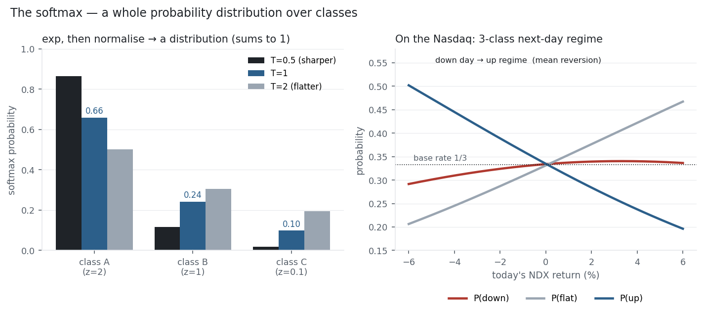
But notice the axis: the three curves only fan out to roughly 0.20–0.50 at the extreme ±6% days, and for a typical day near zero they all sit right on the 1/3 base rate. Softmax is doing exactly what it should — handing back a genuine, normalised distribution over regimes — and the mild tilt it reports is real. It is simply, once again, the honest verdict of a near-efficient market: the shape of the distribution barely departs from the unconditional class frequencies, because today’s return says little about tomorrow’s.

Same multi_daily.csv as the previous entries (yfinance, adjusted closes). The three regimes are equal-sized terciles of the next day’s NDX return; a multinomial logistic regression on the current return gives the softmax probabilities (scikit-learn). Every number was checked.

Common mistakes

• Applying softmax to independent labels. Softmax forces the outputs to sum to 1, so it is for mutually-exclusive classes (pick one); for independent yes/no tags, use a sigmoid per label.
• Forgetting the max-subtraction. Naive softmax overflows for large scores; always subtract the maximum first (or use a library implementation).
• Reading the top probability as accuracy. A softmax output of 0.9 is the model’s confidence, not its correctness; on markets especially, confident and right are different things.
• Interpreting raw logits as probabilities. The scores going in are on an unbounded scale; only after exponentiate-and-normalise are they a distribution.
• Ignoring temperature. The same logits look decisive or unsure depending on T; temperature scaling is how over-confident softmax outputs get calibrated.
• Pairing softmax with squared error. Cross-entropy (next) is the loss that gives softmax its clean gradient; MSE trains it slowly and badly.