Stationarity & the ADF Test
The assumption every model rests on — is the series stable, or is it wandering?
Almost every time-series model — autocorrelation, AR, ARIMA, regression — quietly assumes the series is stationary: that its statistical character does not change over time. Break that assumption and the models do not just lose accuracy, they lie — you can “prove” a strong relationship between two things that have nothing to do with each other. Stationarity is the licence to model, and the Augmented Dickey-Fuller test is how you check for it.
The equation
A series is (weakly) stationary if its mean, variance, and autocovariances do not depend on time:
\mathbb{E}[y_t] = \mu, \quad \text{Var}(y_t) = \sigma^2, \quad \text{Cov}(y_t, y_{t-k}) = \gamma_k \quad \text{for all } t.
The ADF test checks the opposite — whether the series has a unit root — by regressing the change on the level and testing \gamma = 0:
\Delta y_t = \alpha + \beta t + \gamma\, y_{t-1} + \sum_{i=1}^{p}\delta_i\, \Delta y_{t-i} + \varepsilon_t.
The ADF statistic is the t-ratio on \gamma; a sufficiently negative value rejects the unit root and declares the series stationary.
What each symbol means
| Symbol | Meaning |
|---|---|
| y_t | the series at time t |
| \mu,\ \sigma^2 | the constant mean and variance under stationarity |
| \gamma_k | the autocovariance at lag k (depends only on k, not t) |
| \Delta y_t | the first difference, y_t - y_{t-1} |
| \gamma | the coefficient ADF tests; \gamma = 0 means a unit root |
| unit root | the fingerprint of a random walk — non-stationarity |
| p | number of lagged differences added to absorb autocorrelation (“augmented”) |
The ADF null hypothesis is “non-stationary” (has a unit root); a small p-value rejects it in favour of stationarity.
Plain-English explanation
A stationary series looks statistically the same wherever you stand on it: the same average level, the same amount of wobble, the same short-term memory. A non-stationary one drifts — its mean or variance changes over time. Prices are the classic non-stationary series: a stock at 400 has a completely different “average level” than when it was at 40, and its swings grow with its price. Returns are roughly stationary: whatever the price, daily returns hover around a small constant mean with a fairly stable spread. That is why the whole toolkit runs on returns, not prices.
The Augmented Dickey-Fuller test formalises the check. It asks whether the series has a unit root — the fingerprint of a random walk, where shocks never fade and the series wanders with no fixed home. Its null is “unit root / non-stationary”; if the ADF statistic is negative enough (p < 0.05), you reject that and call the series stationary. The “augmented” part just adds lagged differences so ordinary autocorrelation doesn’t fool it. One quirk: because a random walk’s statistics aren’t normal, ADF uses its own (Dickey-Fuller) critical values — more negative than the usual ±1.96, around −2.86 at 5%.
Why it matters in markets
Stationarity is the line between analysis and self-deception, and its most dangerous violation is spurious regression. Take two completely unrelated non-stationary series — two independent random walks — regress one on the other, and you will usually find a “highly significant” relationship with a big R^2. It is an illusion, created entirely by two things wandering, not by any real link. In a simulation of 2,000 such regressions, 84% came back significant at the 5% level — where only 5% should. Ignore stationarity and your t-statistics and p-values become meaningless.
This is why the standard workflow is: difference prices into returns (which are stationary), model those, and ADF-test anything before trusting a regression on it. It is also the gateway to cointegration (the next entry) — the rare case where two non-stationary series share a stationary combination, which is what makes honest pairs trading possible.
A simple worked example
The prices [100, 102, 101, 105, 108, 112] climb — their mean over the first three points (101) is nothing like the mean over the last three (108.3). Non-stationary: the average level depends on when you look. Difference them into changes, [+2, -1, +4, +3, +4], and there is no trend in the level — just fluctuation around a small positive mean. Differencing is the standard cure, and a single difference turns a random-walk price into a stationary return series. The ADF test is what tells you whether you have differenced enough.
Python implementation
from statsmodels.tsa.stattools import adfuller
import pandas as pd

px = pd.read_csv("../multi_daily.csv", index_col="Date", parse_dates=True)["NDX"]

stat_p, p_p = adfuller(px, autolag="AIC")[:2]                        # on prices
stat_r, p_r = adfuller(px.pct_change().dropna(), autolag="AIC")[:2]  # on returns
print(round(stat_p, 2), round(p_p, 3))      # -> 1.39   0.997   prices: unit root (non-stationary)
print(round(stat_r, 2), round(p_r, 3))      # -> -18.09  0.0    returns: stationary
A p-value above 0.05 means “can’t reject a unit root” — treat the series as non-stationary and difference it.
Manual / Excel calculation
There is no clean spreadsheet formula for ADF — it needs a regression with special critical values, so use statsmodels (Python) or R’s tseries::adf.test. What you can do in Excel: plot a rolling mean and a rolling standard deviation. If either trends, the series is non-stationary and needs differencing before any modelling.
Financial-market example — Nasdaq 100
The two panels are the whole idea. NDX’s price wanders from ~4,500 to ~26,000 over the decade — its one-year rolling mean drifts the entire way, and the ADF test agrees emphatically: statistic +1.39, p-value 0.997, nowhere near rejecting a unit root. A textbook random walk with drift.
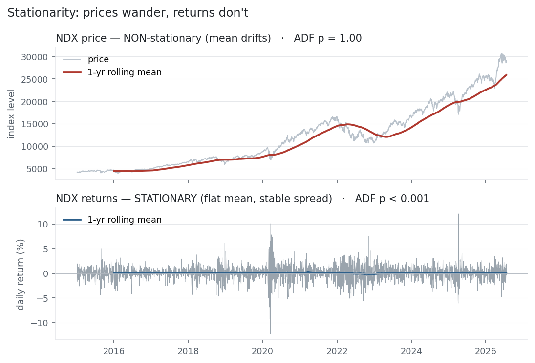
Its returns are the opposite: the one-year rolling mean sits flat against zero (ranging only −0.15% to +0.27%), the spread is broadly stable, and the ADF statistic is −18.1 with a p-value below 0.001 — decisively stationary. Same asset, two completely different statistical worlds, separated by a single difference. This is exactly why every earlier entry computed returns first: mean, volatility, autocorrelation — all of them are meaningful only on the stationary return series, never on the wandering price.
Same multi_daily.csv as the previous entries (yfinance, adjusted closes). ADF via statsmodels; the spurious-regression figure of 84% is a 2,000-run simulation of independent random walks.
Common mistakes
- Modelling raw prices. Prices are non-stationary; regressions and AR models on them are unreliable. Difference to returns first.
- Trusting a regression without an ADF test. A high R^2 between two non-stationary series is very likely spurious — 84% of the time in the simulation above.
- Using normal critical values for ADF. The statistic doesn’t follow the t-distribution under the null; use the Dickey-Fuller values (≈ −2.86 at 5%) or the reported p-value.
- Reading “fail to reject” as “proven non-stationary.” The ADF test has low power; failing to reject can also mean too little data. It is evidence, not proof.
- Over-differencing. Differencing an already-stationary series adds artefacts (spurious negative autocorrelation); difference just enough.
- Assuming stationarity is permanent. Regimes shift; a series stationary in-sample can drift out-of-sample. Re-test.