Value at Risk & Expected Shortfall

The loss you won’t exceed most days — and the average of the days you do

quant finance

risk

VaR and Expected Shortfall (CVaR): the two standard tail-risk numbers. Historical vs Gaussian VaR, why ES is the coherent measure, and a Nasdaq-100 example where the normal model understates the tail.

Author

David Maguire

Maximum drawdown measures the worst loss that already happened; Value at Risk asks a forward question — how bad could an ordinary bad day be? VaR is the loss a portfolio won’t exceed with a given confidence; Expected Shortfall is the average loss on the days it does. Together they are the standard language of tail risk — and, as the fat tails we measured warn, the method you use to estimate them matters enormously.

The equation

VaR at confidence c is the loss threshold breached only with probability 1-c — the negative of the lower quantile of returns. Expected Shortfall is the average return in that tail:

\text{VaR}_c = -\,Q_{1-c}(r), \qquad \text{ES}_c = -\,\mathbb{E}\!\left[\,r \mid r \le Q_{1-c}(r)\,\right]

where Q_{1-c}(r) is the (1-c) quantile of returns (e.g. the 5th percentile for 95% confidence). Both are quoted as positive numbers — losses.

What each symbol means

Symbol	Meaning
\text{VaR}_c	Value at Risk at confidence c — the loss you won’t exceed with probability c
\text{ES}_c	Expected Shortfall (a.k.a. CVaR) — the average loss given a breach of VaR
c	the confidence level (e.g. 95%, 99%)
Q_{1-c}(r)	the (1-c) quantile of returns — the tail cutoff
r	the return series, over the chosen horizon

VaR is a point (the cutoff); ES is an average (of everything worse than the cutoff). So \text{ES}_c \ge \text{VaR}_c always.

Plain-English explanation

Pick a confidence level, say 95%. The 95% VaR is the loss such that only 5% of days are worse — the edge of the “bad but not disastrous” zone. If your one-day 95% VaR is 2%, then on 19 days out of 20 you expect to lose less than 2%; on the 20th, more.

VaR’s fatal flaw is that it says nothing about how bad that 20th day is: a 2% VaR is identical whether the bad days average −2.1% or −20%. Expected Shortfall repairs this — it is the average of all the returns beyond VaR, so it measures how deep the tail actually runs. VaR is “how often”; ES is “how bad when it happens.”

There are two ways to compute them. Historical: just look at what happened — sort the returns and read off the percentile. Parametric: assume a bell curve and use its formula. The two agree only if returns are normal, and they never are.

Why it matters in markets

VaR is everywhere — the number on the risk report, the basis of position limits, and for two decades the regulatory capital standard. But it has two deep flaws that ES repairs. First, VaR ignores tail severity: it is the doorway, not the room, so a book can show a modest VaR and catastrophic losses just beyond it — the blind spot that helped hide risk in 2008. Second, VaR is not coherent: it can violate subadditivity, so a diversified portfolio can post a higher VaR than the sum of its parts, perversely penalising diversification. Expected Shortfall is coherent and tail-sensitive, which is why Basel moved bank capital rules from VaR to ES.

And both live or die by the tail assumption. For the fat-tailed, negatively skewed returns markets actually produce, a Gaussian VaR is dangerously optimistic: it prices the rare disaster as rarer than it is.

A simple worked example

Ten daily returns, sorted: [-6\%,\, -4\%,\, -2\%,\, -1\%,\, 0\%,\, 1\%,\, 1\%,\, 2\%,\, 3\%,\, 5\%]. At 80% confidence, the worst 20% is the two returns -6\% and -4\%. The VaR is the cutoff — the least bad of the tail, -4\%, i.e. an 80% VaR of 4%. The ES is the average of the whole tail, \tfrac{-6\% + (-4\%)}{2} = -5\%, i.e. an ES of 5%. ES exceeds VaR because it counts the −6% day that VaR simply ignores.

Python implementation

import numpy as np
import pandas as pd

r = (pd.read_csv("../multi_daily.csv", index_col="Date", parse_dates=True)
       .pct_change().loc["2025-07-01":"2026-06-30"])["NDX"].dropna()

c = 0.95
q = np.percentile(r, (1 - c) * 100)      # the 5th-percentile return (a loss)
hist_var = -q                             # historical VaR
hist_es  = -r[r <= q].mean()              # historical ES: average of the tail beyond VaR
print(round(hist_var * 100, 2), round(hist_es * 100, 2))   # -> 1.92  2.49

# parametric (Gaussian) VaR assumes a normal distribution
z = 1.6449                                # 95% z-score
par_var = z * r.std(ddof=1) - r.mean()
print(round(par_var * 100, 2))            # -> 1.77   (smaller: the normal ignores fat tails)

Two traps: np.percentile(r, 5) returns the loss quantile, and VaR is its negative; and the Gaussian version needs z = 2.3263 for 99%, not 1.645.

Manual / Excel calculation

Historical: sort the returns; VaR is the (1-c) percentile; ES is the average of everything at or below it. With returns in B2:B252:

Task	Formula
Historical 95% VaR	`=-PERCENTILE.INC(B2:B252, 0.05)`
Historical 95% ES	`=-AVERAGEIF(B2:B252, "<="&PERCENTILE.INC(B2:B252,0.05))`
Parametric 95% VaR	`=1.645*STDEV.S(B2:B252) - AVERAGE(B2:B252)`

Financial-market example — Nasdaq 100

NDX daily returns, same window — one-day VaR and ES, historical against the Gaussian model:

Confidence	historical VaR	historical ES	Gaussian VaR	Gaussian ES
95%	1.92%	2.49%	1.77%	2.25%
99%	2.84%	3.85%	2.55%	2.94%

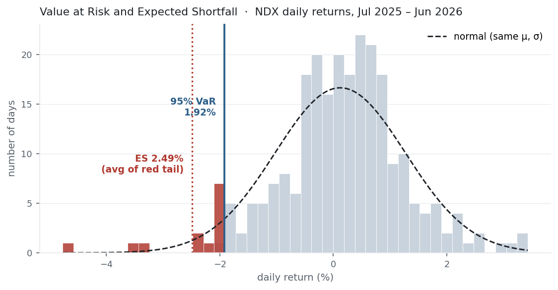
Histogram of NDX daily returns, left tail shaded, with VaR and ES lines and a normal overlay — NDX daily returns with the 95% VaR cutoff (blue) and Expected Shortfall (red, the average of the shaded tail). The tail pokes well outside the normal curve — the fat tail VaR alone can’t see.

On a $1,000,000 position, the one-day 95% VaR is about $19,200 — you’d expect to lose more than that on roughly 1 day in 20 (over the year there were 13 such days out of 251, bang on 5%). Expected Shortfall says that when you do breach it, the average loss is about $24,900.

The fat-tail warning from Skewness & Kurtosis surfaces exactly where it should — deep in the tail. At 99%, the Gaussian model puts ES at 2.94%, but the returns actually delivered 3.85%: the bell curve underestimates the average disaster by nearly a full percentage point (about $29,400 vs $38,500 on the million). VaR looks almost fine under the normal assumption; ES is where the model’s optimism turns dangerous, because that is where the fat tail lives.

Same multi_daily.csv as the previous entries (yfinance, adjusted closes). Code blocks are illustrative — every figure was computed and checked against that file.

Common mistakes

Trusting Gaussian VaR on fat-tailed returns. The normal understates the tail; use historical or a fat-tailed model. At 99% the gap is material.
Reading VaR as a maximum loss. VaR is a threshold you breach (1-c) of the time; losses beyond it are unbounded — which is the whole reason ES exists.
Forgetting VaR isn’t coherent. It can penalise diversification (violate subadditivity); ES doesn’t, which is why regulators switched to it.
Dropping the horizon or confidence. VaR scales with \sqrt{\text{horizon}} (like σ) and is meaningless without stating both the horizon and the confidence level.
Too little data for the tail. A 99% VaR from one year rests on ~2–3 observations; tail estimates are desperately data-hungry.
Confusing VaR and ES. VaR is the cutoff, ES the average beyond it — quote which, and never compare a VaR to an ES.