Variance & Standard Deviation

The second moment — how far returns scatter around their mean, and the root that turns it into risk

Variance and its square root, standard deviation (volatility): the spread of a return series, sample vs population (n−1), √252 annualisation, and a worked Nasdaq-100 example — including the numpy/pandas ddof trap.

Where the mean is the reward, variance and standard deviation are the risk. They measure how far a return series scatters around its mean — the difference between a calm asset and a wild one that share the same average. This is the second thing you compute about any strategy, and the denominator of almost every risk-adjusted number that follows.

The equation

\sigma^2 \;=\; \frac{1}{n-1}\sum_{t=1}^{n}\left(r_t - \bar r\right)^2 \qquad\qquad \sigma \;=\; \sqrt{\sigma^2}

Sample variance is the average squared deviation of returns from their mean, dividing by n-1 rather than n. Standard deviation is its square root — back in the original return units, and in finance the per-period volatility.

What each symbol means

Symbol	Meaning
\sigma^2	the sample variance of returns (spread, in return²)
\sigma	the sample standard deviation / volatility (spread, in return units)
r_t	the return in period t — a simple return, as in Mean Return
\bar r	the sample mean return, \tfrac{1}{n}\sum_t r_t
n	the number of return observations
n-1	Bessel’s correction — dividing by n-1 makes \sigma^2 an unbiased estimate of the true variance

Variance is measured as squared distance from \bar r, so you must compute the mean first — the two statistics are joined at the hip.

Plain-English explanation

Variance asks: on average, how far do the returns land from their mean — squared? Take each return’s distance from the mean, square it (so pluses and minuses don’t cancel, and big misses count for more), and average. Those squared distances are in “return²”, a unit nobody thinks in, so take the square root to get the standard deviation, back in plain return terms. Annualised, that number is what the market calls volatility — the standard measure of risk.

Two assets can share a mean and still feel nothing alike; σ is what separates the steady one from the one that lurches. The mean is the reward; σ is the risk.

Why it matters in markets

σ is the denominator of the entire risk-adjusted-return apparatus: the Sharpe ratio, the \sigma in the volatility-drag relation g \approx \bar r - \tfrac{1}{2}\sigma^2 from Mean Return, the scale of a Value-at-Risk estimate, the key input to option pricing, and the risk term in mean–variance portfolio construction. Size a position, model risk, or compare two strategies, and you are leaning on σ.

One property matters constantly: variance adds over time; volatility scales with its square root. Over h independent periods variance grows like h\sigma^2, so σ grows like \sqrt{h}. That is why you annualise volatility by \sqrt{252}, not 252 — the exact opposite of how the mean scales. Mean return is linear in time; volatility is square-root-of-time.

A simple worked example

The three returns from Mean Return, +2\%,\,-1\%,\,+3\%, with mean \bar r = 1.33\%:

\sigma^2 = \frac{(0.02-0.0133)^2 + (-0.01-0.0133)^2 + (0.03-0.0133)^2}{3-1} = \frac{0.000867}{2} = 0.000433,

so \sigma = \sqrt{0.000433} = 0.0208 = 2.08\%. The returns sit on average about 2.1 percentage points from their 1.33% mean — a spread bigger than the mean itself, which is precisely why the mean alone tells you so little.

Python implementation

import numpy as np
import pandas as pd

r = np.array([0.02, -0.01, 0.03])          # the three returns from the Mean Return entry

# --- sample variance and std, spelled out to match the formula ---------------
mean   = r.mean()                          # r-bar: compute the mean FIRST
sq_dev = (r - mean) ** 2                    # squared distance of each return from the mean
var    = sq_dev.sum() / (r.size - 1)        # divide by n-1 (Bessel) -> SAMPLE variance
std    = var ** 0.5                         # standard deviation = sqrt(variance)
print(round(var, 6), round(std * 100, 4))   # -> 0.000433   2.0817   (sigma = 2.08%)

# --- the catch: numpy and pandas disagree on the DEFAULT divisor -------------
print(round(np.std(r), 4))                  # -> 0.017    numpy default ddof=0 (POPULATION, /n)
print(round(np.std(r, ddof=1), 4))          # -> 0.0208   ddof=1 gives the SAMPLE std (/n-1)
print(round(pd.Series(r).std(), 4))         # -> 0.0208   pandas already defaults to ddof=1

That default mismatch is a genuine bug source: annualise a numpy σ computed with its default and you understate risk by a factor of \sqrt{n/(n-1)}. For daily data with large n the error is tiny; for small samples it is not. For returns, you almost always want the sample version (ddof=1).

Manual / Excel calculation

By hand: (1) mean, (2) each return’s deviation from the mean, (3) square them, (4) sum, (5) divide by n-1, (6) square root.

In Excel, with returns in B2:B4:

Task	Formula
Sample variance	=VAR.S(B2:B4) → 0.000433
Sample std (volatility)	=STDEV.S(B2:B4) → 0.0208
Population versions	=VAR.P(B2:B4), =STDEV.P(B2:B4) (divide by n)
Annualised volatility	=STDEV.S(B2:B4)*SQRT(252)

.S = sample (÷ n-1), .P = population (÷ n). Match the divisor to your Python/pandas choice or the numbers won’t reconcile.

Financial-market example — Nasdaq 100

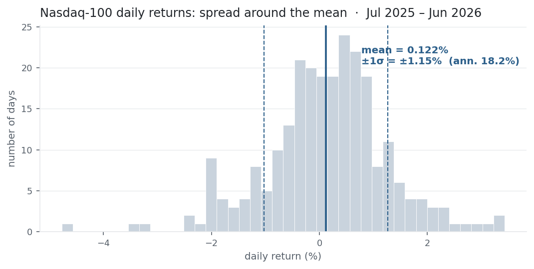
The same window as Mean Return — daily ^NDX returns, 1 Jul 2025 to 30 Jun 2026, n = 251.

Histogram of Nasdaq-100 daily returns over the window, with the mean (solid) and ±1σ (dashed) marked. σ is the width of this cloud; the extra weight in the tails is what a single σ misses.

import pandas as pd, numpy as np

r = (pd.read_csv("../ndx_daily.csv", parse_dates=["Date"])
       .set_index("Date")["Close"].pct_change()
       .loc["2025-07-01":"2026-06-30"])

var = r.var()                      # pandas -> SAMPLE variance (ddof=1)
sd  = r.std()                      # daily volatility (ddof=1)
ann = sd * np.sqrt(252)            # annualised volatility: sigma * sqrt(252)

print(round(var, 8))               # -> 0.00013169   daily variance (return^2)
print(round(sd * 100, 4))          # -> 1.1475       % per day
print(round(ann * 100, 2))         # -> 18.22        % annualised

Daily volatility is 1.15%, i.e. 18.2% annualised (1.15\% \times \sqrt{252}). The daily variance, 0.00013, is in return² — meaningless to eyeball, which is the whole reason we quote σ instead.

The histogram shows two things. σ is a width: about 72.5% of days fall within ±1σ of the mean and 95.6% within ±2σ — close to the 68% / 95% a normal distribution predicts, but not equal. And that gap is informative: the extra mass in the tails (that −4.7% day) is the fat-tailedness a single σ can’t see. Note also \tfrac{1}{2}\sigma^2 \approx 0.0066\% per day here — exactly the volatility drag that split the arithmetic and geometric means in Mean Return.

Same ndx_daily.csv as Mean Return (yfinance, ^NDX). Code blocks are illustrative — the site doesn’t execute them, so every figure was computed and checked against that file.

Common mistakes

• Wrong divisor (n vs n−1). numpy.std defaults to ddof=0 (population, ÷n); pandas.std defaults to ddof=1 (sample, ÷n−1). Mix them and your σ won’t reproduce. For returns, use the sample version.
• Annualising σ with ×252 instead of ×√252. Variance scales with time, volatility with its square root; ×252 overstates annual vol by ~16×. (Mean return does scale by ×252 — σ does not.)
• Trusting one σ for fat-tailed returns. Real returns have heavier tails than the normal, so σ underweights the rare large move. Pair it with skew/kurtosis, VaR, or drawdown before calling it “risk.”
• σ of prices instead of returns. The standard deviation of a trending price series mostly measures the trend, not risk. Always compute σ on returns.
• Confusing variance and volatility units. Variance is in return²; only σ is comparable to returns. Quote σ, reconcile in variance.
• Too short a sample. σ from a few weeks is noisy and regime-dependent — a calm month badly understates the σ of the next crisis.