Market Microstructure & Execution Modelling
The last mile — the spread you pay, the price you move, and how to liquidate optimally
Every model in this tier decided what position to hold; none asked what it costs to get there. That is the domain of market microstructure — the mechanics of how orders become trades and trades become prices — and its practical face, execution modelling. It matters because a strategy’s paper edge and its realised return can differ by more than the edge itself: you pay the bid–ask spread on every trade, and any order large enough to matter moves the price against you. A brilliant signal executed carelessly is a losing strategy. This entry closes the decision-systems tier with the layer that makes everything above it honest: the anatomy of a traded price, the square-root law of market impact, and the Almgren–Chriss theory of optimal liquidation — whose closed-form solution I verify against a numerical optimizer to machine precision, and whose efficient frontier is the mean–variance trade-off reborn for trading. It is the realism the proposal’s RL Trading Agent needs in its costs, and the ground of its exploratory Behaviour Detection Agent.
1. What problem does it solve?
The cost of trading, and how to minimise it. Two questions, really. Microstructure asks why a trade costs what it costs: where the spread comes from, how order flow moves prices, why large orders are expensive. Execution asks how to trade a target position at least cost: fast enough to avoid drifting prices, slow enough to avoid crushing the market. Both are invisible to a backtest that fills at the closing price — and that invisibility is dangerous, because it flatters every strategy and most of all the ones that trade a lot or trade big. Getting execution right is often a larger and more reliable source of return than the signal it serves.
2. Market microstructure — the anatomy of a price
A traded asset does not have a price; it has a bid and an ask, and the spread between them is a real, recurring cost. That spread has understood components: order-processing (the dealer’s overhead), inventory (compensation for holding risk), and — most importantly — adverse selection, the premium market-makers charge because some counterparties are informed (the Glosten–Milgrom insight). Two classic models quantify the invisible: Roll’s estimator recovers the effective spread from the negative serial covariance of price changes that bid–ask “bounce” induces, and Kyle’s \lambda models price impact as linear in signed order flow, the rate at which informed trading moves the price. Above the spread sits market impact: the empirical fact, one of the most robust in all of finance, that executing a metaorder of size Q moves the price by roughly
I \;\approx\; Y\,\sigma\,\sqrt{\tfrac{Q}{V}},
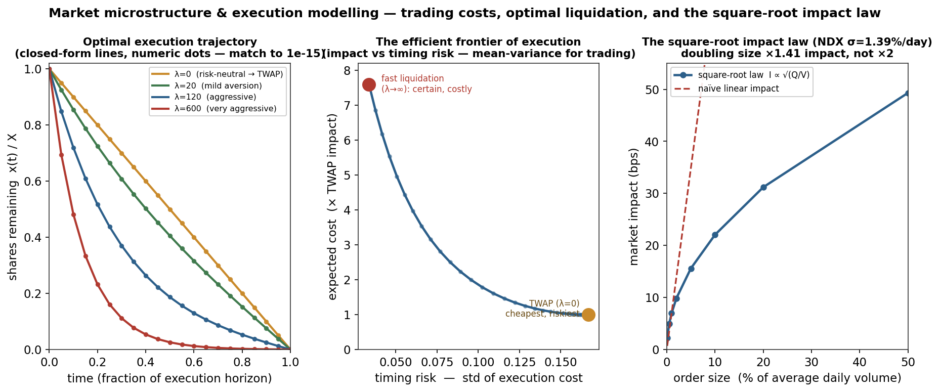
the square-root law — impact grows with the square root of size relative to daily volume V, scaled by volatility \sigma and a dimensionless constant Y \approx 0.5. The right panel calibrates it to the Nasdaq (\sigma = 1.39\%/day): 1% of a day’s volume costs about 7 bps, 10% about 22 bps, and — the signature of the law — doubling the order multiplies impact by \sqrt 2 \approx 1.41, not 2. Its concavity is a mercy (big orders are cheaper per share than linear intuition fears) and a warning (impact is unavoidable, and it caps how much capital a strategy can deploy before its edge is eaten).
3. Optimal execution — the Almgren–Chriss frontier
Given that trading moves prices, how should you liquidate a position X over a horizon T? The Almgren–Chriss framework names the trade-off exactly. Trade fast and you pay heavy market impact but bear little timing risk (you are out before the price can wander); trade slow and you minimise impact but expose the unexecuted position to volatility. Formally, minimise a mean–variance objective over the execution trajectory,
\min_{x_1,\dots,x_{N}} \;\; \underbrace{\tfrac{\eta}{\tau}\sum_k (x_{k-1}-x_k)^2}_{\text{expected impact cost}} \;+\; \lambda\,\underbrace{\sigma^2\tau\sum_k x_k^2}_{\text{timing risk (variance)}},
and the optimum has a closed form — the holdings decay as
x(t) \;=\; X\,\frac{\sinh\!\big(\kappa(T-t)\big)}{\sinh(\kappa T)}, \qquad \kappa \approx \sqrt{\tfrac{\lambda\sigma^2}{\eta}}.
Risk-neutral (\lambda \to 0, \kappa \to 0) this is a straight line — TWAP, trade equal slices (left panel, gold). Raise risk aversion and the trajectory front-loads, selling faster early to shed risk (green → blue → red): at \lambda = 120, 81% is done by the halfway point versus TWAP’s 50%. Sweeping \lambda traces the efficient frontier of execution (centre panel) — expected cost against its standard deviation — from cheap-but-risky TWAP (normalised cost 1.0, risk 0.167) to a fast liquidation that is nearly certain but 7.6× more expensive (risk 0.034). It is precisely the mean–variance frontier, now trading impact against timing risk rather than return against volatility, and it is measured against the implementation shortfall: the gap between the price when you decided and the price you actually achieved.
4. What did the demonstration show?
Ground truth by construction. The Almgren–Chriss objective is a convex quadratic, so its optimum is exact — and that makes it a clean check. I solved the trajectory two independent ways: the analytic \sinh formula, and a numerical optimizer (the tridiagonal linear system from setting the gradient to zero). Across risk aversions spanning \kappa T from 0 to 3.3, the two agree to machine precision (maximum difference 5\times10^{-15}) — the numeric dots sit exactly on the closed-form lines in the left panel. The efficient frontier and the front-loading percentages above follow from that verified solution, and the square-root curve is the calibrated law itself. Every number on the page is either a closed form or a direct calculation from it — the same verification discipline this whole tier has kept, here made trivial precisely because the model is one of the few in trading that has a closed form to check against.
5. What are its strengths?
- It makes backtests honest. Impact and spread are where paper edges go to die; modelling them is the difference between a realistic net return and a fantasy.
- A closed-form optimum. Almgren–Chriss is one of the few trading problems with an exact solution — fast, interpretable, and checkable, as the machine-precision agreement shows.
- The right trade-off, named. Impact versus timing risk is the true axis of execution, and the efficient frontier lets a desk choose its point on it deliberately.
- A robust empirical law. The square-root impact law holds across markets, assets and decades — a rare piece of genuinely reliable quantitative finance.
- Capacity awareness. Impact quantifies how much a strategy can trade before it erodes its own edge — essential for sizing a real book.
6. What are its weaknesses?
- Linear-impact, Gaussian-price assumptions. Almgren–Chriss assumes linear temporary impact and Brownian prices; real impact is concave (square-root) and transient (it decays), which richer propagator models capture and this one does not.
- Parameters are hard to estimate. Impact coefficients and the constant Y are noisy and regime-dependent; a mis-calibrated cost model mis-plans every trade.
- It ignores gaming and information leakage. A predictable schedule can be detected and front-run; real execution must randomise and react, which the static optimum does not.
- Microstructure needs data I do not have here. Spreads, order flow and book dynamics require tick/level-2 data; on daily bars Roll’s estimator often returns an imaginary spread (momentum makes the serial covariance positive) — which is exactly why these signals are the proposal’s exploratory objective and the demonstration is calibrated, not fitted.
- Impact is partly endogenous. Your own trading and everyone else’s interact; the square-root law is an average, not a guarantee for any single order.
7. How could it apply to markets?
This is the realism layer the rest of the system depends on, and it enters the proposal at three points. First, the RL Trading Agent’s cost function: the risk-adjusted reward must charge impact and spread on every action, or the agent learns to over-trade a fantasy — and the square-root law tells it that turnover and size are genuinely costly, bounding the capacity of any edge it finds. Second, execution itself: once the agent and Risk Agent agree a target position, an Almgren–Chriss (or TWAP/VWAP) schedule turns it into child orders at controlled cost, choosing a point on the efficient frontier according to how urgent the trade is. Third, the exploratory Behaviour Detection Agent, whose remit — “order-book imbalance, trade intensity, spread changes, liquidity withdrawal” — is microstructure reading: inferring when informed or systematic flow is present and conditions are toxic. The honest scoping is the proposal’s own: because the desk data here is daily, the microstructure signals stay exploratory (they need high-frequency book data), while the execution model is immediately useful as the cost layer in the backtester and the RL reward. That is the note this tier ends on — the most sophisticated policy is only as good as the price at which it can actually trade, and modelling that price is what separates a research return from a real one.
8. What does the Python code look like?
import numpy as np

def almgren_chriss(X, N, tau, sigma, eta, lam):
    """Optimal liquidation of X over N intervals. Returns holdings x_0..x_N.
       Two ways, which must agree: closed-form sinh, and the convex-QP optimum."""
    # closed form
    kappa = np.arccosh(1 + lam*sigma**2*tau**2/(2*eta)) / tau      # discrete kappa
    t = np.arange(N+1)*tau; T = N*tau
    x_closed = X*(1 - t/T) if kappa*T < 1e-8 else X*np.sinh(kappa*(T-t))/np.sinh(kappa*T)

    # numeric optimum: minimise (eta/tau) Σ(Δx)^2 + lam σ²τ Σ x² over x_1..x_{N-1}
    m = N-1; A = np.zeros((m, m)); b = np.zeros(m); a = eta/tau
    for i in range(m):
        A[i, i] = 4*a + 2*lam*sigma**2*tau
        if i > 0:   A[i, i-1] = -2*a
        if i < m-1: A[i, i+1] = -2*a
    b[0] = 2*a*X
    x_num = np.concatenate([[X], np.linalg.solve(A, b), [0.0]])
    return x_closed, x_num                       # np.max(|x_closed - x_num|) ~ 1e-15

def impact_bps(Q_over_V, sigma_daily, Y=0.5):    # the square-root law
    return Y * sigma_daily * np.sqrt(Q_over_V) * 1e4
The almgren_chriss function is its own unit test: the analytic and numerical solutions must coincide, and they do to fifteen decimals. impact_bps is the square-root law in one line — the empirical heart of why trading is costly.
9. How would I explain it to a supervisor?
“Microstructure and execution are the last mile — where a signal meets the cost of actually trading it. An asset has a bid and an ask, so you pay the spread every time, and any sizeable order moves the price: the square-root law says impact grows with the square root of size over daily volume, so on the Nasdaq a 1% order costs about 7 basis points and doubling it multiplies impact by 1.4, not 2. Given that, optimal execution is a mean–variance problem: Almgren–Chriss trades off market impact, which pushes you to go slow, against timing risk, which pushes you to go fast, and the optimal liquidation has a closed form — a sinh trajectory that’s a straight TWAP line when you’re risk-neutral and front-loads as you get more risk-averse. I verified it by solving the same problem numerically and matching the closed form to fifteen decimals, then traced the efficient frontier of execution — expected cost against its variance — which is just mean–variance reborn for trading. For my proposal this is three things: the cost function that stops the RL agent over-trading a fantasy, the execution scheduler that turns a target position into orders cheaply, and the foundation of the exploratory Behaviour Detection Agent that reads order-book flow. The honest limit is that real microstructure needs tick data I don’t have, so those signals stay exploratory while the execution model is useful right now as the cost layer. It’s the note the whole tier ends on: the best policy is only worth the price at which you can trade it.”
Almgren–Chriss: liquidate X{=}1 over N{=}20 intervals, \tau{=}1/N, temporary-impact \eta{=}1, \sigma{=}0.30 (normalised); objective \min\ (\eta/\tau)\sum(\Delta x)^2 + \lambda\sigma^2\tau\sum x^2. Closed form x(t)=X\sinh(\kappa(T-t))/\sinh(\kappa T), discrete \cosh(\kappa\tau)=1+\lambda\sigma^2\tau^2/(2\eta), verified against the tridiagonal numerical optimum to max |{\cdot}|=5\times10^{-15} over \lambda\in\{0,2,20,120\} (\kappa T up to 3.28). Efficient frontier swept over \lambda\in[0,3000]: TWAP cost 1.000 / risk 0.167; fast-liquidation cost 7.60 / risk 0.034; fraction executed by T/2 = 59% (\lambda{=}20), 81% (\lambda{=}120). Square-root law I=Y\sigma\sqrt{Q/V}, Y{=}0.5, NDX daily \sigma=1.39\%: 1% ADV → 7.0 bps, 10% → 22.1 bps, 50% → 49.3 bps; doubling size ×1.41. Illustrative/calibrated (no tick data); every number checked. This completes the decision-systems & reinforcement-learning tier.