Do Calendar Anomalies Survive Honest Scrutiny?
A multiple-testing discipline check — 29 seasonal effects, and what’s left after Bonferroni and out-of-sample
The Monday effect, turn-of-month, sell-in-May, the January effect — calendar anomalies are the classic hunting ground for spurious patterns. Testing 29 of them on the Nasdaq and applying honest corrections, exactly one clears p<0.05 (fewer than chance predicts), none survive multiple-testing correction, and it fails to replicate out of sample. A worked demonstration of the discipline the whole site runs on.
Research question
Calendar anomalies — the Monday effect, the turn-of-month effect, “sell in May,” the January effect, the Santa Claus rally — are the oldest and most seductive patterns in markets, and the classic way to fool yourself with data. There are dozens of them, each cheap to test, and with enough tests something will always look significant. So this experiment is less about the calendar than about method: if you hunt seasonal effects honestly — testing a whole battery, correcting for the number of tests, and demanding out-of-sample replication — how many are left? It is the applied companion to the backtest-overfitting demonstration, run on real anomalies instead of simulated ones, and a direct test of the capstone’s third finding: that most apparent edges are methodology lying to you.
Hypothesis
H₀ (mine): essentially nothing survives. Given the number of calendar effects one can define, a handful will clear p < 0.05 by chance alone; after a multiple-testing correction and an out-of-sample check, I expected zero robust anomalies — consistent with the near-efficiency this site has found at every turn. The interesting question was not whether the null would hold but how cleanly — whether the data would show the textbook signature of pure noise.
Data & method
Daily Nasdaq-100 returns, 2015–2026 (multi_daily.csv). I defined a battery of 29 calendar effects — the five weekdays, the twelve months, several turn-of-month windows, first-versus-second half of the month, sell-in-May, the January / September / Santa seasonals, options-expiration Friday, and a few conditional rules (e.g. Monday after a down Friday). Each effect is a group of days; for each I ran a Welch t-test of the mean return on those days against all others, collecting the effect size (bp/day), the t-statistic and the p-value.
The honesty is in the correction. I report (i) how many effects clear p < 0.05 raw, against the 0.05N expected by chance; (ii) how many survive Bonferroni (p < 0.05/N) and Benjamini–Hochberg false-discovery-rate control; (iii) the observed maximum |t| against \sqrt{2\ln N}, the expected maximum of N pure-noise tests (the same \sqrt{2\ln N} that governed the deflated Sharpe ratio); and (iv) an out-of-sample replication — whether effects significant in the first half of the data stay significant, same-signed, in the second.
Results
The null holds, and it holds with the textbook signature of noise. Of the 29 effects, exactly one clears p < 0.05 raw — options-expiration Friday, at p = 0.008 — and that is already fewer than the 1.5 false positives you would expect from 29 independent tests at the 5% level. Under Bonferroni (p < 0.0017) none survive; under Benjamini–Hochberg FDR control, none survive. And the tell is exact: the largest t-statistic in the whole battery is 2.69, sitting almost precisely on \sqrt{2\ln 29} = 2.60 — the biggest result is not evidence of an anomaly, it is exactly what the maximum of 29 coin-flips looks like.
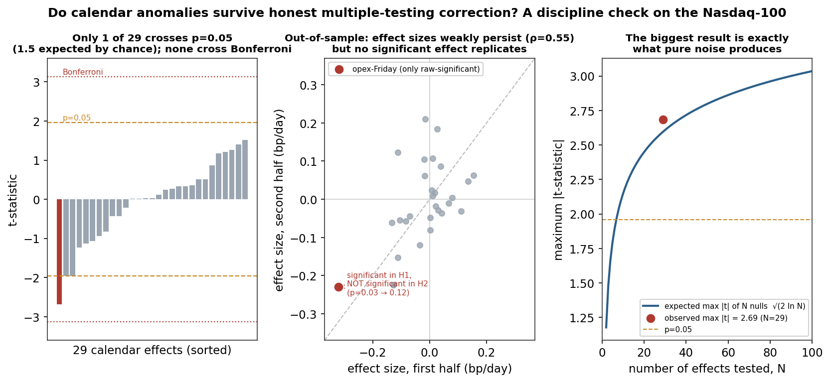
And it fails out of sample. Split the decade in half and the one raw-significant effect does not replicate: options-expiration Friday goes from p = 0.03 in the first half to p = 0.12 in the second — no longer significant. Of the effects significant in the first half, zero replicated as significant and same-signed in the second. The honest nuance is that the effect sizes are weakly correlated across the two halves (ρ = 0.55) — the general shape of seasonal returns is not pure noise, there is faint structure — but it is far too small and too fragile to be a tradeable anomaly, and none of it clears the bar once you account for having looked 29 times. Even the one persistent candidate, the small negative options-Friday return, is 0.28 bp/day — under a third of a basis point, comfortably inside transaction costs.
The verdict
No calendar anomaly on the Nasdaq survives honest scrutiny. The single effect that looks significant is (1) fewer than chance predicts from 29 tests, (2) has a t-statistic exactly at the noise maximum, (3) dies under both Bonferroni and FDR correction, and (4) is not significant out of sample. This is not a failure to find something — it is a clean, positive demonstration that the method works: the same battery run without correction would have handed me “the options-expiration Friday effect, significant at the 1% level” as a finding, and it would have been an artifact. That is precisely the trap the capstone names as the third way a backtest lies, here caught in the act on the most classic of anomaly-hunting grounds.
It is also the right bookend for the Quant Lab. The other five experiments asked whether sophisticated ideas — volatility timing, regime conditioning, risk limits — earn their keep, and answered with careful yeses and noes. This one asks whether a naive idea survives naive testing, and answers with a disciplined no — which is the foundation the careful answers rest on. A lab that cannot reliably reject a false anomaly cannot be trusted when it accepts a true one.
Limitations
- The 29 effects are correlated, so the effective number of independent tests is smaller than 29 — Bonferroni is conservative here. But the conclusion (nothing survives) is on the safe side of that error, and the raw count already undershoots chance.
- Daily data, one index, one decade. A longer history or intraday seasonality could reveal genuine microstructure effects (the options-Friday sign is persistent, if tiny); the claim is “not tradeable and not correction-surviving here,” not “no calendar structure exists anywhere.”
- Welch t-tests assume weak dependence. Returns are close to serially uncorrelated (established across the site), so this is mild, but a block bootstrap would be the fully rigorous version.
- I chose the 29 effects, which is itself a researcher degree of freedom — though a larger battery would only raise the expected max-|t| bar, making survival harder, not easier.
What I learned
The reusable lesson is the one the whole lab is built to internalise: the honest number of trials is the whole story. “Options-expiration Friday has significantly negative returns, p = 0.008” is a true sentence and a false finding — true because the test says so, false because it is one of twenty-nine tests and the best of twenty-nine coin-flips looks just like this. Correcting for the count, and demanding that a result survive into data it was not found in, is the difference between research and a well-dressed guess. That this experiment produced nothing is exactly why it belongs here: it is the control that makes the lab’s positive results — volatility’s forecastable half-life, regime-conditioning’s calibration edge, hard limits’ viability — worth believing.
References
- Bailey, D. H., & López de Prado, M. (2014). The Deflated Sharpe Ratio. Journal of Portfolio Management, 40(5).
- Harvey, C. R., Liu, Y., & Zhu, H. (2016). … and the Cross-Section of Expected Returns. Review of Financial Studies, 29(1).
- Sullivan, R., Timmermann, A., & White, H. (2001). Dangers of Data Mining: The Case of Calendar Effects in Stock Returns. Journal of Econometrics, 105(1).
- Benjamini, Y., & Hochberg, Y. (1995). Controlling the False Discovery Rate. Journal of the Royal Statistical Society B, 57(1).
29 calendar effects tested on daily NDX returns (2015–2026) by Welch t-test. Raw p < 0.05: 1 (options-expiration Friday, −0.28 bp/day, t = −2.69, p = 0.008) vs 1.5 expected by chance; Bonferroni (p < 0.0017): 0; Benjamini–Hochberg FDR: 0. Observed max |t| = 2.69 vs √(2 ln 29) = 2.60. Out-of-sample: effect-size correlation ρ = 0.55 across halves; 0 of 1 first-half-significant effects replicate (opex-Friday p = 0.03 → 0.12). Computed from equations/multi_daily.csv, verified in the sandbox.