ARIMA
The Box-Jenkins synthesis — autoregression, differencing and moving average in one model
ARIMA is where this section’s threads tie together. It stacks the three ideas you’ve just met — autoregression on past values, a moving average of past shocks, and the differencing that turns a wandering price into a stationary series — into one forecasting model. Its three parameters (p, d, q) are a recipe: difference d times to kill the trend, then explain what is left with p autoregressive and q moving-average terms. It is the workhorse of classical time-series forecasting, and applied honestly to a near-efficient market it delivers a sobering verdict.
The equation
ARIMA(p, d, q) applies d differences and then fits an ARMA(p, q):
\Delta^d y_t = c + \underbrace{\sum_{i=1}^{p}\phi_i\, \Delta^d y_{t-i}}_{\text{AR: past values}} + \varepsilon_t + \underbrace{\sum_{j=1}^{q}\theta_j\, \varepsilon_{t-j}}_{\text{MA: past shocks}}
\Delta y_t = y_t - y_{t-1} is the first difference; \Delta^d applies it d times.
What each symbol means
| Symbol | Meaning |
|---|---|
| y_t | the original (possibly non-stationary) series |
| \Delta^d | differencing d times — the “I” (integrated) part |
| p | AR order — number of past values |
| d | number of differences needed to reach stationarity |
| q | MA order — number of past shocks |
| \phi_i,\ \theta_j | AR and MA coefficients |
| c | constant / drift term |
| \varepsilon_t | white-noise shock |
The three orders map to three diagnostics: d from a stationarity test, p from the PACF, q from the ACF.
Plain-English explanation
ARIMA is a three-step recipe for a series that won’t sit still. First the “I”: difference the series d times until it is stationary — for a price, one difference (today minus yesterday) turns it into returns, which are stationary. Then the “AR” and “MA”: model the differenced series as a mix of its own recent values (AR) and its own recent shocks (MA). Put together, ARIMA(p,d,q) says “difference d times, then explain the result with p lags of itself and q lags of noise.”
The three numbers are chosen, not guessed. d is how many differences the ADF test needs to call the series stationary (usually 0 for returns, 1 for prices). Then, on the differenced series, the shape of the correlogram picks p and q: an ACF that cuts off after q and a PACF that cuts off after p — the identification rule from the AR and MA entries. Fit by maximum likelihood, compare candidates by AIC, and check the residuals are white noise. Many familiar models are just corners of this cube: ARIMA(0,1,0) is a random walk with drift, ARIMA(1,0,0) is AR(1), ARIMA(0,0,1) is MA(1), ARIMA(0,1,1) is exponential smoothing.
Why it matters in markets
ARIMA is the classical forecasting workhorse — demand, rates, economic series — but its lesson for markets is the honest capstone of this whole section. Run the full Box-Jenkins machine on the Nasdaq and it confirms, from the inside, that the index is very close to a random walk with drift. It will happily fit AR and MA terms to the faint −0.12 autocorrelation the last four entries kept finding, and AIC will even prefer them — but the forecast it produces is a drift line wrapped in an uncertainty cone that widens as \sqrt{\text{horizon}} (the same √time law). You can forecast the expected drift and the range of outcomes; you cannot forecast the path. That is not a failure of ARIMA — it is ARIMA correctly reporting that the level of a near-efficient price is unforecastable.
It is also the launchpad for what ARIMA can’t do. It models the mean of the differenced series and assumes constant-variance shocks — but returns have clustering volatility (the squared-return autocorrelation). Modelling that time-varying variance is the job of GARCH, the next entry, which bolts onto an ARIMA mean like a second engine.
A simple worked example
The “I” is the only new mechanic, so make it concrete. Prices [100, 102, 101, 105] are non-stationary (they trend), so difference once: [+2, -1, +4] — the changes, a stationary series you can model with ARMA. Suppose that ARMA fit forecasts the next change as +1.5. To get back to a price you integrate (undo the difference): add it to the last level, 105 + 1.5 = 106.5. That round trip — difference to model, integrate to forecast — is the whole idea of the “I”, and it is why a d=1 forecast of a level is always “last value plus the forecast of the change.”
Python implementation
from statsmodels.tsa.arima.model import ARIMA
import numpy as np, pandas as pd

lp = np.log(pd.read_csv("../multi_daily.csv", index_col="Date", parse_dates=True)["NDX"])

fit = ARIMA(lp.values, order=(2, 1, 1), trend="t").fit()   # (p,d,q) on log price
fc  = fit.get_forecast(90)                                  # 90-day-ahead forecast
mean, ci = fc.predicted_mean, fc.conf_int(alpha=0.05)       # point + 95% band
print(round(fit.aic, 1)) # -> -16603.6 (AIC)order=(p,d,q); trend="t" adds the drift. pmdarima.auto_arima automates the order search, but always eyeball the residual ACF — a good ARIMA leaves white noise behind.
Manual / Excel calculation
ARIMA isn’t a spreadsheet job — the MA part needs maximum likelihood — but the Box-Jenkins workflow is followable anywhere: (1) difference the series and ADF-test until stationary → d; (2) read the ACF and PACF of the differenced series to pick q and p; (3) fit with statsmodels / R and compare AIC; (4) confirm the residuals are white noise (Ljung-Box). The one piece you can do by hand is differencing and integrating (=B3-B2, and a running total to undo it).
Financial-market example — Nasdaq 100
Walk the recipe on NDX log price. The ADF test can’t reject a unit root in the level (p = 0.94) but crushes it after one difference (p < 0.001), so d = 1 — the price is I(1), exactly as the stationarity entry found. Scanning ARIMA(p,1,q) for p, q \le 2, AIC picks ARIMA(2,1,1), beating the plain random walk ARIMA(0,1,0) by 47 AIC points — the AR and MA terms are real, soaking up the same lag-1 structure this section keeps meeting.
| Model | AIC | reading |
|---|---|---|
| ARIMA(0,1,0) — random walk + drift | −16,557 | the baseline |
| ARIMA(2,1,1) — best fit | −16,604 | +47 AIC: real but small structure |
And yet look at what the “best” model actually forecasts:
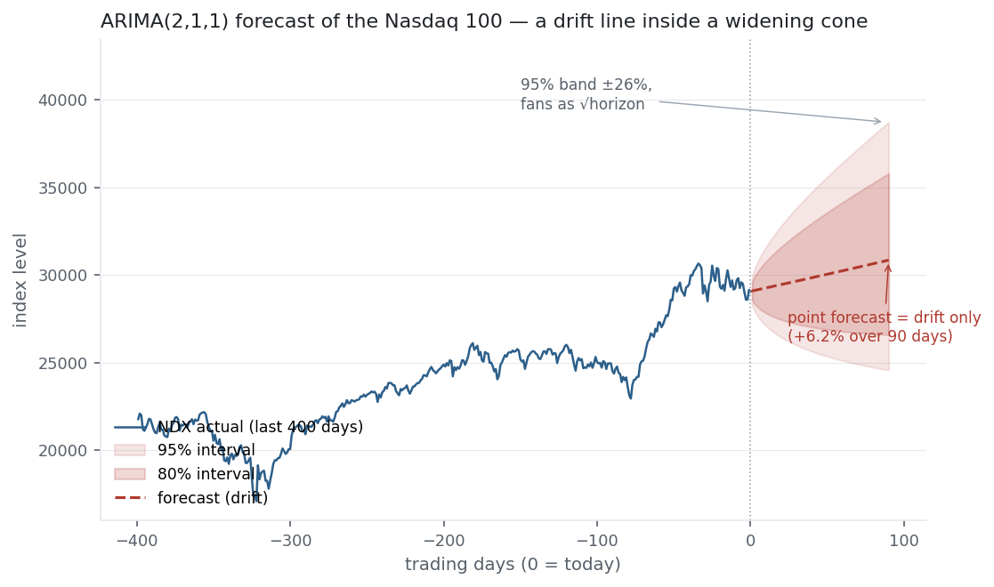
The point forecast is just the drift — +6.2% over 90 days (16.6%/yr) — and the 95% band is ±26%, fanning out as \sqrt{\text{horizon}} (9× wider at 90 days than at 1, and \sqrt{90} \approx 9.5). The AR and MA terms AIC liked so much move only the first few days by a fraction of a percent; by any horizon you’d trade on they have washed out, and the forecast is indistinguishable from a random walk with drift. That is the efficient-market hypothesis in the language of forecasting: you can know the drift and the uncertainty, but the path of a near-efficient index is noise.
Same multi_daily.csv as the previous entries (yfinance, adjusted closes); ARIMA via statsmodels, orders scanned by AIC, forecast on log price then mapped back to level. Code blocks are illustrative — every number was computed and checked.
Common mistakes
- Skipping the stationarity check for d. Under-differencing leaves a trend that corrupts the fit; let the ADF test set d, don’t guess.
- Over-differencing. Too high a d injects artefacts (a spurious −1 lag-1 autocorrelation); d = 1 is almost always enough for a price.
- Reading in-sample AIC as forecast skill. A model can win AIC by 47 points and still forecast the level no better than a random walk — check out-of-sample.
- Not diagnosing the residuals. If the residual ACF isn’t white noise the order is wrong; a good ARIMA leaves nothing behind.
- Expecting ARIMA to capture volatility. It models the mean with constant-variance shocks; clustering volatility needs GARCH.
- Trusting long-horizon point forecasts. Beyond a few steps an ARIMA forecast collapses to the drift; the interval, not the point, is the information.