Beta, CAPM & Alpha

Market risk, the return it should earn, and whatever is left over

Beta as sensitivity to the market, CAPM’s prediction of expected return from beta, and alpha as the miss. Systematic vs idiosyncratic risk, the Security Market Line, and a Nasdaq-100 basket including a negative-beta name.

Covariance told us how two assets move together. Beta specialises that to the one relationship that dominates finance: how an asset moves with the market. From beta, CAPM builds a prediction of what return an asset should earn, and alpha is whatever it earns beyond that. Together they are the foundation of asset pricing and the whole language of systematic versus stock-specific risk.

The equation

Three linked equations. Beta is an asset’s covariance with the market over the market’s variance:

\beta_i = \frac{\text{Cov}(r_i, r_m)}{\text{Var}(r_m)} = \rho_{im}\,\frac{\sigma_i}{\sigma_m}

CAPM turns beta into an expected return:

\mathbb{E}[r_i] = r_f + \beta_i\left(\mathbb{E}[r_m] - r_f\right)

and alpha is the actual return minus what CAPM predicted:

\alpha_i = \bar r_i - \left[\,r_f + \beta_i(\bar r_m - r_f)\,\right]

What each symbol means

Symbol	Meaning
\beta_i	beta — the asset’s sensitivity to the market (slope of its returns on the market’s)
r_i,\ r_m	the asset’s and the market’s returns
\rho_{im}	their correlation
\sigma_i,\ \sigma_m	their volatilities
r_f	the risk-free rate
\mathbb{E}[r_m] - r_f	the market risk premium
\alpha_i	alpha — return earned above (or below) CAPM’s prediction

The market’s own beta is 1 by construction (\text{Cov}(r_m, r_m)/\text{Var}(r_m) = 1). A beta of 1.3 means the asset tends to move 1.3× the market; 0 means no market link; negative means it moves against the market.

Plain-English explanation

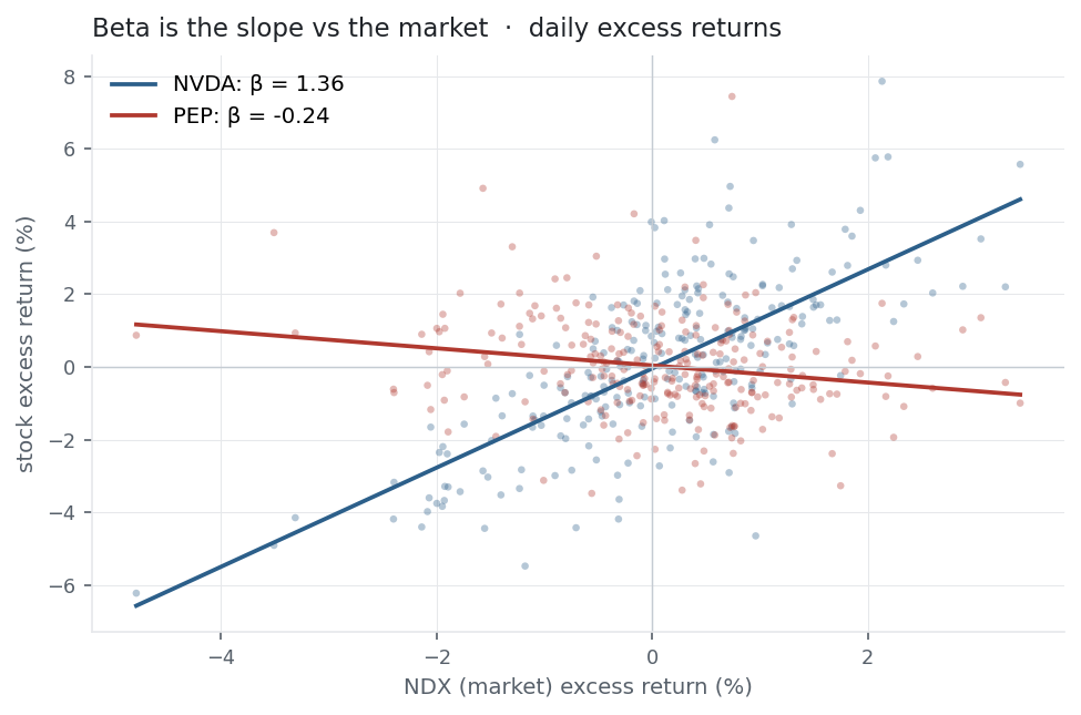
Beta answers: when the market moves 1%, how much does this asset move? It is the slope of the asset’s returns plotted against the market’s. Beta 1 moves with the market, 2 amplifies it two-for-one, 0.5 dampens it, and below 0 moves opposite — a hedge.

CAPM then makes a bold claim: the only risk you are paid for is market risk (beta), because everything else — stock-specific risk — you can diversify away for free. So an asset’s fair expected return is the risk-free rate plus its beta times the market’s risk premium. High-beta assets should earn more (they hurt most when the market falls); a zero-beta asset should earn only the risk-free rate.

Alpha is the verdict: what an asset actually delivered minus what CAPM said it should. Positive alpha beat the model (skill, luck, or a missing risk factor); negative fell short. Chasing alpha is the entire active-management industry.

Why it matters in markets

Beta splits risk into two kinds, and that split is the central idea of portfolio theory. Systematic risk (beta) is shared with the market and cannot be diversified away, so it must be compensated; idiosyncratic risk is stock-specific and vanishes in a large portfolio, so CAPM says it earns nothing. R^2 — the square of the correlation with the market — measures how much of an asset’s variance is systematic; the rest is its own.

Beta is also the hedge ratio: short \beta units of the market against a long position to neutralise market exposure — the basis of market-neutral strategies. And alpha, the CAPM residual, is the benchmark every active manager is judged against — though a positive alpha may simply mean your one-factor model is missing a factor, which is exactly how multi-factor models (Fama–French and the rest) were born.

A simple worked example

A market series r_m = [-2\%, +1\%, +1\%] and an asset r_i = [-4\%, +1\%, +3\%] (both with mean 0):

\beta = \frac{\sum (r_i-\bar r_i)(r_m-\bar r_m)}{\sum (r_m-\bar r_m)^2} = \frac{(-4)(-2)+(1)(1)+(3)(1)}{(-2)^2+1^2+1^2} = \frac{12}{6} = 2.0.

The asset amplifies the market two-for-one — a beta of 2. If the risk-free rate is 0 and the market is expected to return 1%, CAPM predicts this asset should earn 0 + 2\,(1\% - 0) = 2\%.

Python implementation

import numpy as np
import pandas as pd

r = (pd.read_csv("../multi_daily.csv", index_col="Date", parse_dates=True)
       .pct_change().loc["2025-07-01":"2026-06-30"])
m = r["NDX"]                                    # market proxy

beta = r["NVDA"].cov(m) / m.var()               # beta = Cov(asset, market) / Var(market)
print(round(beta, 2))                            # -> 1.36

# CAPM expected return and alpha (annualised, rf = 4%)
rf, A = 0.04, 252
prem  = m.mean() * A - rf                         # market risk premium
capm  = rf + beta * prem
alpha = r["NVDA"].mean() * A - capm
print(round(capm * 100, 1), round(alpha * 100, 1))   # -> 40.4  -10.3

# beta is also the slope of the stock regressed on the market
print(round(np.polyfit(m, r["NVDA"], 1)[0], 2))      # -> 1.36  (same number)

cov/var and the regression slope are the same beta. Alpha is simply what is left once beta has explained everything it can.

Manual / Excel calculation

Beta is a slope; CAPM and alpha are one line each. With market returns in A2:A252 and the stock in B2:B252:

Task	Formula
Beta	=SLOPE(B2:B252, A2:A252)  (or =COVARIANCE.P(B2:B252,A2:A252)/VAR.P(A2:A252))
CAPM expected return	=0.04 + Beta*(market_annual - 0.04)
Alpha	=stock_annual - CAPM_expected

SLOPE regresses the stock on the market — the y-argument is the stock, the x-argument the market. Get them the wrong way round and you compute the market’s beta to the stock instead.

Financial-market example — Nasdaq 100

Each basket name regressed on the NDX index (the market), same window. The market premium was 26.7% over r_f = 4\%:

Ticker	beta	R^2	actual	CAPM	alpha
NVDA	1.36	0.49	30.1%	40.4%	−10.3%
MSFT	0.54	0.13	−24.4%	18.3%	−42.7%
AAPL	0.53	0.17	37.7%	18.1%	+19.6%
PEP	−0.24	0.04	8.8%	−2.3%	+11.1%
NDX	1.00	1.00	30.7%	30.7%	0.0%

The Security Market Line: CAPM’s predicted return for each beta (dashed). Each asset’s vertical distance from the line is its alpha — AAPL and PEP above it, NVDA and MSFT below.

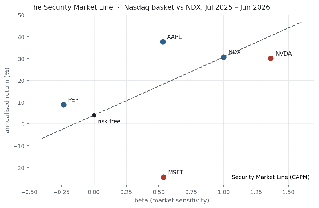
Three things stand out. NVDA is the only high-beta name (1.36) — it is a huge index weight, so nearly half its variance (R^2 = 0.49) is the market and the rest is its own story. PEP has a negative beta (−0.24), a consumer-staples name drifting against the tech tape — the closest thing here to a hedge. And look at the alphas: they are enormous and all over the place (AAPL +20%, MSFT −43%). Over a single year, “alpha” is overwhelmingly noise — with R^2 this low the market explains only a sliver of each stock, and the residual is mostly luck. That is the honest lesson of CAPM on real data: beta is estimable, alpha is treacherous. On the Security Market Line, CAPM’s prediction is the dashed line and each asset’s distance from it is its alpha; the scatter is exactly why one window proves nothing.

To measure how beta is estimated — the slope of the stock’s returns against the market’s — here are NVDA (steeply positive) and PEP (slightly negative) on the same axes:

Daily excess returns of NVDA and PEP against the market. Beta is the slope: NVDA’s line rises at 1.36, PEP’s falls at −0.24.

Same multi_daily.csv as the previous entries (yfinance, adjusted closes). Code blocks are illustrative — every figure was computed and checked against that file.

Common mistakes

• Reading alpha as skill. Over short windows alpha is dominated by noise; a year of data can’t tell a skilled manager from a lucky one.
• Forgetting beta needs a benchmark. Beta is always relative to a chosen market; a stock’s beta to the Nasdaq differs from its beta to the S&P or its sector.
• Treating CAPM as truth. It is a one-factor model with famously mixed empirical support — low-beta stocks have historically out-earned it (the low-beta anomaly), and missing factors masquerade as alpha.
• Confusing high beta with high return. Beta predicts sensitivity, not realised return — NVDA’s high beta didn’t stop it undershooting CAPM here.
• Ignoring R^2. A beta with R^2 = 0.04 (PEP) barely means anything; the market explains almost none of that stock’s movement.
• Estimating from too little. Beta is computed from returns and drifts over time; a short, noisy sample gives an unstable number.