The Cost Function
The thing a model minimises — how learning becomes optimisation
Everything in machine learning starts here. A model has knobs — its parameters — and a cost function is the single number that says how badly those knobs are set: how far the model’s predictions sit from the truth. “Training” is nothing more than turning the knobs to make that number as small as possible. So the cost function is what converts a vague goal (“predict well”) into a precise mathematical problem (“minimise J”), and everything that follows in this section — gradient descent, mean squared error, cross-entropy, regularisation — is either a choice of cost or a way to minimise one.
The equation
A cost function J aggregates a per-example loss L over the training data:
J(\theta) = \frac{1}{n}\sum_{i=1}^{n} L\big(y_i,\ \hat y_i(\theta)\big)
For squared-error loss, L(y, \hat y) = (y - \hat y)^2, and J is the mean squared error; the parameters \theta that minimise J define the trained model.
What each symbol means
| Symbol | Meaning |
|---|---|
| J(\theta) | the cost — one number scoring the whole model |
| \theta | the model’s parameters (the knobs training turns) |
| L(y, \hat y) | the per-example loss |
| y_i | the true value for example i |
| \hat y_i(\theta) | the model’s prediction, which depends on \theta |
| n | the number of training examples |
Loss is per-example; cost is the average; the objective is often cost plus a regularisation penalty.
Plain-English explanation
A cost function is a scorecard for a model. You feed it the model’s parameters, it makes predictions on your data, compares them to the truth, and returns a single number: high if the predictions are bad, low if they are good. Learning is the search for the parameters that make that number smallest — which is why people say machine learning is “just” optimisation. The trained model is whatever set of knobs sits at the bottom of the cost.
Two words often blur together. The loss is the error on one example (how wrong this single prediction was); the cost is the loss averaged over the whole dataset (how wrong the model is overall). Minimise the cost and you have trained the model. The figure shows the idea at small scale: with one parameter the cost is a curve (a parabola) and training slides to the bottom; with two it is a surface, a bowl whose lowest point is the answer; with a million — a neural network — it is a landscape in a million dimensions, and the whole game is getting down to a low valley.
Why it matters in markets
The cost function is the most consequential design choice in a model, because it defines what “good” means — and the model will optimise exactly what you wrote down, not what you meant. Choose squared error and you penalise big misses quadratically, so the model bends to avoid outliers (and inherits their leverage); choose absolute error and every mistake counts linearly, a more robust fit; choose cross-entropy and you punish confident wrong probabilities savagely. Same data, different cost, different model. In a trading context this is where you encode what you actually care about — a cost that penalises a missed crash more than a missed rally builds a different model than symmetric squared error, and getting that objective wrong is how a backtest that “minimised error” still loses money.
The shape of the cost also decides how hard the optimisation is. For a linear model with squared error the cost is convex — a single bowl with one global minimum, solvable in closed form (it is the OLS solution the figure’s right panel sits at). For a neural network it is wildly non-convex — a rugged landscape of many local minima and saddle points — with no formula for the bottom, which is exactly why iterative methods like gradient descent exist.
A simple worked example
Predict three numbers [2, 4, 6] with a single constant c, under squared-error cost J(c) = \frac{1}{3}\sum (y_i - c)^2. Try c = 3: the errors are [-1, 1, 3], squared [1, 1, 9], mean 3.67. Try c = 5: errors [-3, -1, 1], mean 3.67 again. Try c = 4: errors [-2, 0, 2], squared [4, 0, 4], mean 2.67 — lower. Four is the mean of the data, and that is no coincidence: the constant that minimises squared-error cost is always the mean. The cost function turned “find the best constant prediction” into “find the minimum of a parabola,” and the answer fell out as a familiar statistic.
Python implementation
import numpy as np

def cost(params, X, y):
    y_hat = X @ params                  # model predictions (linear here)
    return np.mean((y - y_hat) ** 2)    # mean squared-error cost

# a constant model's cost is a parabola, minimised at the mean:
r = ...                                 # NDX daily returns
c_grid = np.linspace(r.mean() - 1, r.mean() + 1, 100)
J = [np.mean((r - c) ** 2) for c in c_grid]     # min is exactly at r.mean()
The cost is just a function of the parameters; training hands it to an optimiser. Everything downstream — the loss you pick, the penalty you add — is a modification of this one function.
Manual / Excel calculation
A cost is a column of errors reduced to one number. Put predictions beside actuals, take the difference, square it (=(A2-B2)^2) or take its absolute value, and average the column (=AVERAGE(...)) — that average is the cost. Change the model’s parameter, watch the number move; the parameter that gives the smallest number is the least-squares fit (LINEST finds it directly for a linear model).
Financial-market example — Nasdaq 100
Two costs on the Nasdaq basket make it concrete. First, the simplest possible model: predict every NDX daily return with one constant c. The squared-error cost J(c) = \text{mean}((r - c)^2) is the left parabola in the figure, and it bottoms out at c = 0.08\%/day — the sample mean return — with a minimum cost equal to the return variance itself. The mean is not just a summary statistic; it is the solution to a cost-minimisation problem.
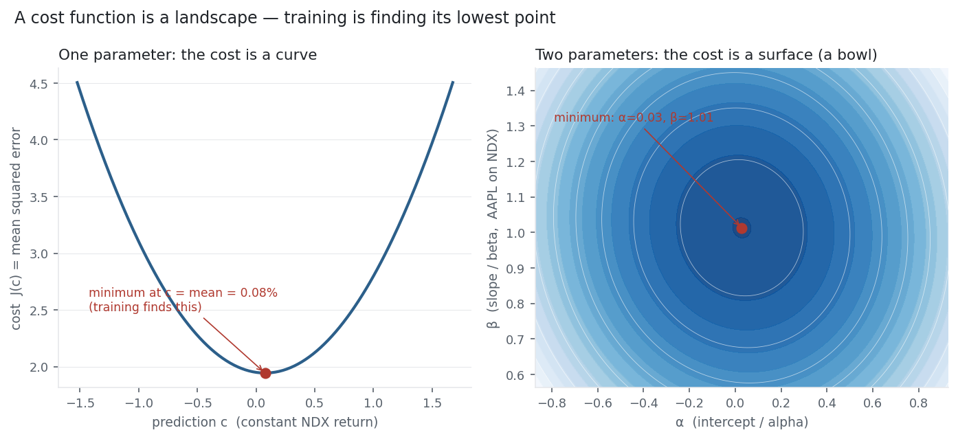
Second, a two-parameter model: predict AAPL’s daily return from the NDX return, \hat y = \alpha + \beta\, r_{\text{NDX}}. Now the cost J(\alpha, \beta) is a surface — the right panel’s bowl — and its lowest point sits at \alpha = 0.03\%/day and \beta = 1.01, which is exactly the CAPM regression of AAPL on the index. Every regression, every trained model, is a point at the bottom of a cost like this. The difference between models is only how many parameters the bowl has and how rugged it is — and, when there is no closed-form bottom, how you climb down. That descent is the next entry.
Same multi_daily.csv as the previous entries (yfinance, adjusted closes). Both costs are mean squared error on daily percent returns; the two-parameter minimum is the OLS regression of AAPL on NDX. Every number was computed and checked.
Common mistakes
- Confusing loss and cost. Loss is per-example error; cost is the average (often plus a penalty). You minimise the cost, not any single loss.
- Optimising the wrong objective. The model minimises the cost you wrote, not the goal you intended; a mis-specified cost is optimised faithfully into a useless model.
- Assuming every cost is convex. Linear-model squared error is a single bowl; neural-net costs are rugged with many minima — “just minimise it” hides very different difficulty.
- Forgetting the cost’s units and scale. Squared error is in squared units and outlier-sensitive; comparing costs across models or scalings without care is meaningless.
- Leaving out regularisation. The training cost isn’t always the whole objective — a penalty term (coming up) trades fit for simplicity to fight overfitting.
- Reading a low training cost as success. Low cost on training data can mean overfitting; the honest score is the cost on data the model never saw.