Gini Impurity

How mixed a node is, without the logarithms — the default splitting criterion of CART trees

Gini impurity = 1 − Σp²: the chance of mislabelling a random sample by a node’s class mix. Binary 2p(1−p), why CART/scikit-learn default to it, how it compares to entropy, and an honest Nasdaq split.

Entropy measures a node’s uncertainty with logarithms; Gini impurity measures the same mixedness with a simpler formula and no logs, which is why it is the default splitting criterion in CART decision trees and scikit-learn. It answers a slightly different question — “if I labelled a random sample by the node’s class frequencies, how often would I be wrong?” — but the answer traces almost the same curve as entropy, and, just as the previous entry’s information gain has a Gini twin, trees built on either usually make the same cuts.

The equation

For a node with class proportions p_1, \dots, p_K:

\text{Gini} = 1 - \sum_{i=1}^{K} p_i^2

For two classes this is 2p(1-p). Gini is 0 when the node is pure (one class) and maximal (0.5 for two classes, 1 - 1/K in general) when the classes are evenly mixed.

What each symbol means

Symbol	Meaning
Gini	the Gini impurity of the node
p_i	proportion of class i in the node
K	number of classes
\sum p_i^2	probability two random draws share a class
1 - \sum p_i^2	probability they differ — the impurity

Plain-English explanation

Gini impurity asks: reach into a node, draw a sample at random, and label it by drawing a class at random from the node’s own frequencies — how often would that label be wrong? If the node is pure (all one class) you’re never wrong, impurity 0. If it’s a 50/50 mix you’re wrong half the time, impurity 0.5. In general the chance of a mismatch is 1 minus the chance of a match, and the chance two independent draws match is \sum p_i^2, giving \text{Gini} = 1 - \sum p_i^2. It is, in a phrase, the expected error rate of guessing by the node’s own class mix.

For two classes the formula collapses to 2p(1-p) — a downward parabola that peaks at p = 0.5 (value 0.5) and hits zero at both ends. That is the same inverted-U as binary entropy, just lower and smoother: the figure overlays them, and half the entropy curve almost lands on the Gini curve. The practical difference is the missing logarithm. Entropy needs a log per class; Gini needs only squares, so it is cheaper to compute across the millions of candidate splits a tree evaluates — which is why CART and scikit-learn reach for Gini by default. A tree scores a split by its Gini gain, parent Gini minus the sample-weighted Gini of the children, exactly as information gain does with entropy.

Why it matters in markets

Gini impurity is the workhorse purity measure inside decision trees, random forests, and gradient-boosted trees — the model families that win a large share of real tabular-data problems in finance. Every split those models make is chosen (by default) to drop Gini the most, and the “feature importances” they report are sums of Gini reductions. So knowing what Gini is means knowing what a tree is actually optimising when it decides that, say, the VIX matters more than the day of the week.

The reassuring news, and the reason to learn it alongside entropy rather than instead, is that the two almost never disagree. On the same Nasdaq split search from the last entry, Gini gain and entropy gain line up on a near-perfect straight line — the two criteria rank every candidate split identically. That means the choice between them is about speed and convention, not results, and the honest verdict they return is the same one this section keeps reaching: applied to tomorrow’s direction from today’s return, the best split any tree could make barely moves either measure.

A simple worked example

Ten samples, 5 up and 5 down: the node is maximally mixed, so \text{Gini} = 1 - (0.5^2 + 0.5^2) = 0.5. Split them 4-up/1-down on the left and 1-up/4-down on the right. Each child is an 80/20 mix, with \text{Gini} = 1 - (0.8^2 + 0.2^2) = 1 - 0.68 = 0.32; weighting the two equally gives a child Gini of 0.32. The Gini gain is 0.5 - 0.32 = 0.18. (Entropy scored the identical split at a gain of 0.28 bits — different number, same ordering, because the two impurities agree on which splits are good.)

Python implementation

import numpy as np

def gini(y):
    _, c = np.unique(y, return_counts=True); p = c / c.sum()
    return 1 - (p**2).sum()

def gini_gain(y, mask):
    n = len(y); yl, yr = y[mask], y[~mask]
    return gini(y) - (len(yl)/n*gini(yl) + len(yr)/n*gini(yr))

# sklearn's default: DecisionTreeClassifier(criterion="gini")

Note this is not the Gini coefficient of income inequality — same name, different quantity; the tree version is the impurity above.

Manual / Excel calculation

Per node, Gini is =1 - SUMSQ(proportions) — for two classes, =1-p^2-(1-p)^2 or simply =2*p*(1-p). A split’s Gini gain is the parent’s Gini minus the sample-weighted sum of the children’s — the same arithmetic as information gain, with squares in place of logs.

Financial-market example — Nasdaq 100

The Nasdaq’s tomorrow-up/down node has class proportions 0.56/0.44, so its Gini impurity is 2 \cdot 0.56 \cdot 0.44 = 0.493 — just shy of the 0.5 maximum, the same near-total mixedness that gave it 0.99 bits of entropy. Search every threshold on today’s return for the split that lowers Gini the most, and the best gain is 0.0005 — about a tenth of one percent of the parent impurity.

Left: Gini 2p(1−p) (max 0.5) and entropy H(p) (max 1 bit) are the same inverted-U — half the entropy curve nearly lands on Gini. Right: each dot is one NDX split, Gini gain vs entropy gain — a straight line (correlation 1.00), every point within a whisker of the origin.

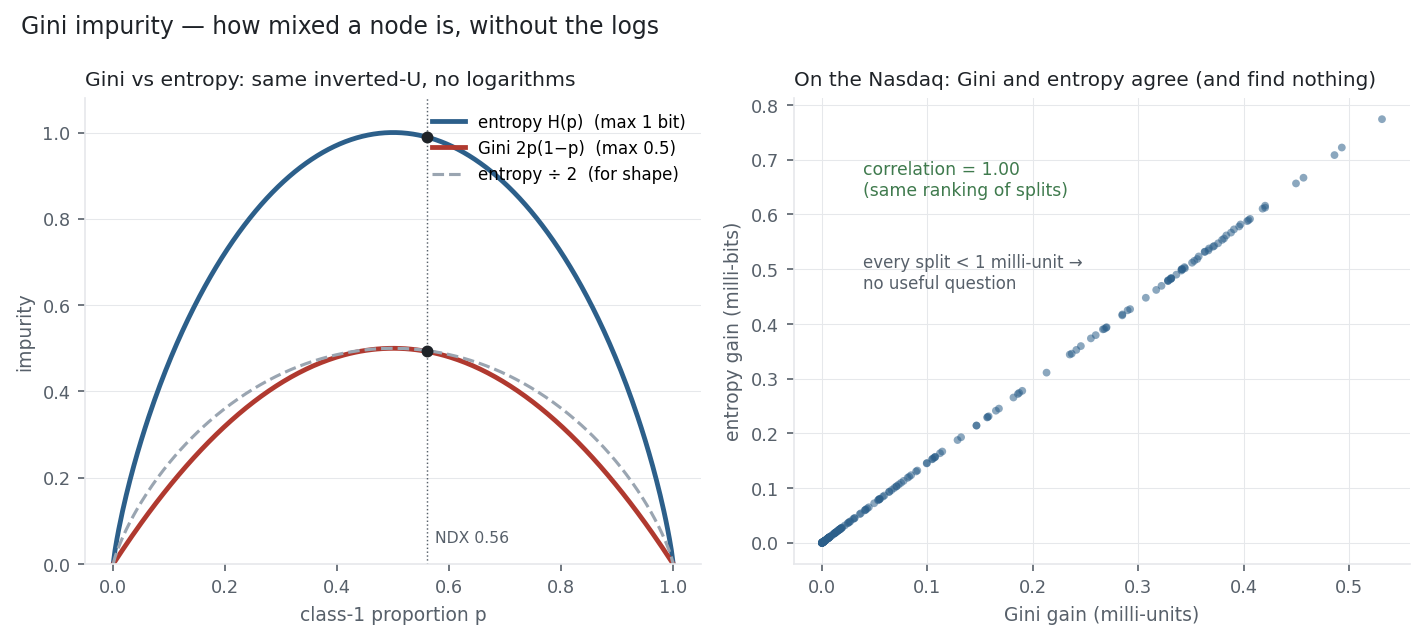
The right panel is the point of this entry. Each dot is one candidate split, its Gini gain against its entropy gain; they fall on a straight line with correlation 1.00, so the two criteria would build the identical tree. And every dot sits within a whisker of the origin — no split, by either measure, meaningfully purifies the node. Gini and entropy, the two tools a tree can choose between, look at the Nasdaq’s next day and return the same answer the rest of this section did: there is almost nothing to split on. The choice of impurity measure is a detail; the absence of signal is the finding.

Same multi_daily.csv as the previous entries (yfinance, adjusted closes). The parent is tomorrow’s NDX up/down node (Gini 0.493, entropy 0.99 bits); gains are scanned over thresholds on today’s return with each child kept ≥ 50 samples. Gini/entropy gain correlation = 1.00. Every number was checked.

Common mistakes

• Confusing it with the Gini coefficient. The impurity here (1 - \sum p^2) is unrelated to the income-inequality Gini coefficient; they only share a name.
• Expecting a maximum of 1. Two-class Gini caps at 0.5, not 1; the general cap is 1 - 1/K.
• Thinking Gini and entropy give different trees. They rank splits almost identically (correlation ≈ 1 here); the pick is about speed, not accuracy.
• Reading impurity as the model’s error rate. Gini is the error of random labelling by the node’s mix, a proxy for purity — not the trained tree’s accuracy.
• Forgetting to weight the children. Gini gain uses the sample-weighted child impurity, like information gain.
• Trusting Gini-based importances blindly. Like information gain, Gini importance inflates high-cardinality features; cross-check with permutation importance.