L1 & L2 Penalties (Lasso & Ridge)
Two ways to penalise weights — sparse feature selection vs smooth shrinkage
Regularisation adds a penalty on complexity; L1 and L2 are the two penalties that do it, and they differ in a way that matters. Both charge for large weights, but L2 (Ridge) charges the square of each weight and L1 (Lasso) charges the absolute value — and that small change flips the behaviour. L2 shrinks every weight smoothly toward zero but never quite to zero; L1 drives weak weights exactly to zero, which turns regularisation into automatic feature selection. Same goal, two personalities.
The equation
The two penalties, each added to the loss and scaled by \lambda:
\underbrace{R_{L2}(\theta) = \sum_i \theta_i^2}_{\text{Ridge (L2 norm)}} \qquad\qquad \underbrace{R_{L1}(\theta) = \sum_i |\theta_i|}_{\text{Lasso (L1 norm)}}
Ridge penalises the squared weights; Lasso penalises their absolute values. Elastic Net uses a mix of the two.
What each symbol means
| Symbol | Meaning |
|---|---|
| \theta_i | the i-th model weight |
| \sum \theta_i^2 | L2 penalty — sum of squared weights (Ridge) |
| \sum |\theta_i| | L1 penalty — sum of absolute weights (Lasso) |
| \lambda | the strength, multiplying the penalty in the objective |
| \|\theta\|_2,\ \|\theta\|_1 | the L2 and L1 norms |
Plain-English explanation
Picture the two penalties as forces pulling every weight toward zero. L2’s pull is proportional to the weight: a big weight feels a strong tug, a small weight barely any — so as a weight shrinks the force fades, and it glides toward zero but never lands. The result is smooth shrinkage: Ridge keeps all your features, just quieter. L1’s pull is constant: every nonzero weight feels the same fixed tug toward zero regardless of size, so a weight the data doesn’t strongly support gets pushed all the way to exactly zero and stays there. The result is sparsity: Lasso throws features out.
The geometry in the figure is the cleanest way to see it. Fitting a model means finding the point of lowest loss inside a “budget” region set by the penalty. L2’s budget is a circle; L1’s is a diamond. Because a circle is smooth, the lowest-loss point on it is almost never on an axis, so both weights stay nonzero. Because a diamond has sharp corners that sit exactly on the axes, the lowest-loss point tends to land on a corner — and a corner means one weight is exactly zero. Stretch to many dimensions and the diamond’s corners are whole subspaces where most weights vanish, which is why L1 zeros out features while L2 doesn’t. In one dimension it is even simpler: L2 gives \theta = z/(1+\lambda) (divide, never zero), L1 gives \theta = \text{sign}(z)\max(|z|-\lambda,\ 0) — subtract a fixed amount and clip at zero, the “soft-threshold.”
Why it matters in markets
The choice between them is a modelling decision with real consequences, especially in finance where you often have far more candidate signals than usable ones (the backtest-overfitting trap). Lasso (L1) is the tool when you believe only a handful of features truly matter and you want the model to tell you which — it produces a short, interpretable list and a sparse model, at the cost of arbitrarily dropping one of any two correlated features. Ridge (L2) is the tool when your features are collinear or all weakly informative and you want a stable fit — it keeps everything, spreads weight sensibly across correlated inputs, and has a clean closed-form solution, at the cost of never simplifying. When you want both, Elastic Net blends them: L1 for selection, L2 for stability among correlated features.
On markets, the honest lesson from the last entry sharpens here. Run Lasso across the 20 lagged Nasdaq returns and, as the penalty rises, it prunes features one by one — 20, then a handful, then none. At the strength that actually generalises, the surviving set is essentially empty: Lasso, asked which past returns predict the next, answers “none of them.” Ridge reaches the same verdict more quietly, shrinking all twenty coefficients toward zero without ever committing to a deletion. L1 states the efficient-market result as an explicit, empty feature list; L2 states it as universal shrinkage. Two penalties, one conclusion.
A simple worked example
Take a single weight the data wants to set to z = 5, and add each penalty at strength \lambda. Ridge minimises (\theta - 5)^2 + \lambda\theta^2, solved by \theta^* = 5/(1 + \lambda): at \lambda = 1 it’s 2.5, at \lambda = 4 it’s 1.0, at \lambda = 8 it’s 0.56 — shrinking, always positive. Lasso minimises (\theta - 5)^2 + \lambda|\theta|, solved by the soft-threshold \theta^* = \max(5 - \lambda,\ 0): at \lambda = 1 it’s 4, at \lambda = 3 it’s 2, and at \lambda = 5 it hits exactly 0 and stays there. Same weight, same strengths — Ridge divides the estimate down, Lasso subtracts a fixed amount and then deletes it.
Python implementation
from sklearn.linear_model import Ridge, Lasso, ElasticNet
import numpy as np

Ridge(alpha=1.0).fit(X, y)                      # L2: all coefficients shrink, none exactly 0
lasso = Lasso(alpha=0.1).fit(X, y)              # L1: many coefficients become exactly 0
ElasticNet(alpha=0.1, l1_ratio=0.5).fit(X, y)   # a blend of both

print(np.sum(lasso.coef_ != 0), "features kept")   # L1 selects a subset
alpha is \lambda; for Elastic Net l1_ratio sets the L1/L2 mix. Scale features first — both norms act on the raw coefficients, so unscaled features are penalised unequally.
Manual / Excel calculation
The shrinkage rules are one-liners once you have the unpenalised estimate z. Ridge: =z/(1+lambda). Lasso (soft-threshold): =SIGN(z)*MAX(ABS(z)-lambda, 0). Fill a column of coefficients through those formulas and you reproduce, per weight, exactly what Ridge and Lasso do to a fit.
Financial-market example — Nasdaq 100
Take the 20-lagged-returns model from the regularisation entry and swap the penalty. Ridge keeps all 20 coefficients at every strength, quietly shrinking them; the figure’s Lasso line tells the other story — as \lambda rises it zeros the coefficients one at a time, 20 → a dozen → three → none.
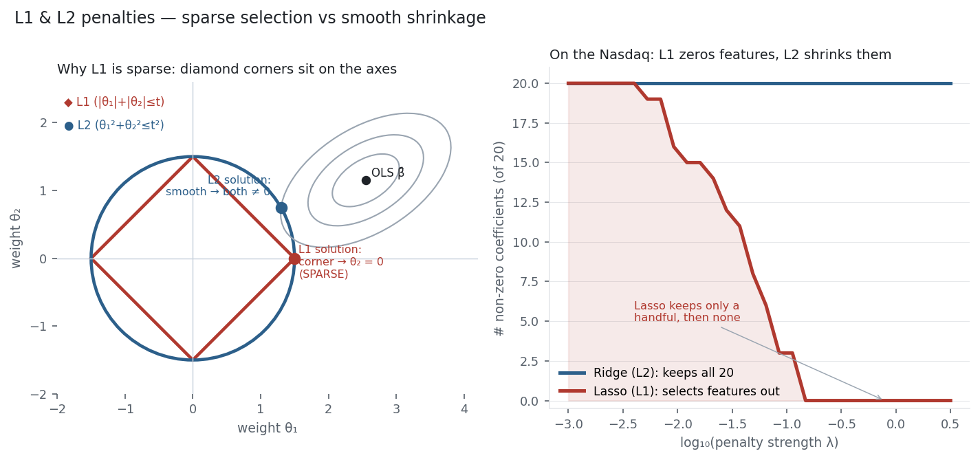
At a weak penalty Lasso still keeps a scatter of lags (largely fitting noise, since the earlier entries showed no lag carries real signal); at the penalty that generalises best — which, for these features, is a heavy one — it keeps essentially nothing. That empty selection is L1’s version of the verdict this whole section keeps returning: presented with twenty candidate predictors of tomorrow’s Nasdaq return, the honest model chooses zero of them. Ridge agrees, having pushed all twenty coefficients to a whisper. The two penalties are different instruments; on a near-efficient market they play the same note.
Same multi_daily.csv as the previous entries (yfinance, adjusted closes). The market panel counts non-zero coefficients of scikit-learn Lasso vs Ridge on 20 standardised lagged NDX returns. The geometry panel is the standard schematic. Every number was checked.
Common mistakes
- Not scaling features. Both penalties act on raw coefficients, so a feature on a larger scale is penalised less; standardise before fitting.
- Expecting Ridge to zero features. L2 shrinks but never sets coefficients exactly to zero; only L1 (or Elastic Net) does selection.
- Trusting Lasso’s pick among correlated features. Lasso keeps one of a correlated group and drops the rest arbitrarily; Elastic Net or domain judgement is safer for selection.
- Reading a kept feature as significant. Lasso keeping a lag at a loose \lambda is not evidence it predicts anything — validate out of sample.
- Penalising the intercept. As with all regularisation, leave the bias term out of the penalty.
- Confusing penalty type with strength. The type sets the shape (sparse vs smooth); \lambda still sets how much — tune it separately by cross-validation.