Regularisation
Penalising complexity to fight overfitting — trading a little bias for a lot less variance
The cost function entry promised that the training objective isn’t always the whole story — that a penalty term often rides alongside the loss. Regularisation is that term. It adds a charge for complexity to the objective, so minimising it no longer means fitting the training data as closely as possible, but fitting it well while staying simple. The reason is the deepest failure mode in machine learning and the cardinal sin of quant finance: overfitting. A model flexible enough to explain every wiggle in the training data has usually learned the noise, and it falls apart on data it hasn’t seen. Regularisation is the standard cure.
The equation
The regularised objective adds a penalty R on the parameters, scaled by \lambda:
J(\theta) = \underbrace{\text{Loss}(\theta)}_{\text{fit the data}} + \lambda\,\underbrace{R(\theta)}_{\text{stay simple}}
\lambda \ge 0 sets the strength: 0 recovers the plain loss; larger \lambda pulls harder toward simplicity. The penalty R is usually a norm of the weights — \sum\theta^2 for L2 (Ridge), \sum|\theta| for L1 (Lasso).
What each symbol means
| Symbol | Meaning |
|---|---|
| J(\theta) | the regularised objective (what training minimises) |
| \text{Loss}(\theta) | the data-fit term (e.g. MSE or cross-entropy) |
| \lambda | regularisation strength (a hyperparameter) |
| R(\theta) | the complexity penalty on the parameters |
| \theta | the model’s parameters (weights) |
Plain-English explanation
Left alone, a training algorithm makes the loss as small as it can — and a model with enough parameters can drive the training loss to nearly zero by contorting itself through every data point, noise included. That contortion is overfitting: the fit looks brilliant on the data it was trained on and terrible on anything new. Regularisation stops it by adding a cost for using large or numerous parameters, so the optimiser only “spends” complexity where it genuinely lowers the loss. The result is a smoother, simpler model that captures the signal and ignores the noise (the figure’s left panel: the flexible fit chases every point and whips out of control, while the regularised fit tracks the underlying shape).
The knob is \lambda, and it sets a tradeoff. At \lambda = 0 there is no penalty and the model is free to overfit — low bias, high variance, great on training data, poor on test. As \lambda grows it forces the parameters toward zero, making the model simpler and steadier — higher bias, lower variance — until, in the limit, it ignores the features entirely and predicts a constant. Somewhere in between is the \lambda that generalises best, and because you cannot see it on the training loss (which only ever rises with \lambda), you find it on held-out validation data. This is the bias-variance tradeoff made adjustable: regularisation lets you dial in exactly how much flexibility the data can support.
Why it matters in markets
In markets, regularisation is not a nicety — it is survival, because financial data is the worst case for overfitting: many candidate features, short history, and a signal-to-noise ratio so low that a flexible model will almost always find convincing patterns that are pure chance. This is the mechanism behind backtest overfitting: search enough strategies or features and some will fit the past beautifully and fail live. Regularisation fights back by charging for complexity up front, biasing the model toward the null — smaller positions, fewer active features, predictions closer to the base rate — which is exactly the humility a near-efficient market rewards.
The Nasdaq experiment in the figure makes the point at its bluntest. Feed a Ridge regression the last 20 daily returns to predict the next, and with no regularisation it earns a positive R^2 on the training window and a negative one out of sample — it literally does worse than predicting the average, the signature of overfitting. Crank \lambda up and the out-of-sample R^2 climbs back toward zero as the coefficients shrink to nothing; the best generalising model is the maximally regularised one, which has learned to predict the mean. Regularisation didn’t just improve the model — it correctly concluded that the twenty features carry no signal, and the right thing to do with noise is ignore it.
A simple worked example
Strip it to one parameter. Suppose the data wants \theta = 5 (that value alone minimises the loss (\theta - 5)^2), but you add an L2 penalty \lambda\theta^2. The regularised objective is (\theta - 5)^2 + \lambda\theta^2, and setting its derivative to zero gives \theta^* = 5/(1 + \lambda). At \lambda = 0 you get \theta = 5, the unregularised answer. At \lambda = 1 it halves to 2.5; at \lambda = 4, down to 1; at \lambda = 99, just 0.05. The penalty shrinks the estimate toward zero, and more so the stronger it is — every regularised weight is a compromise between what the data wants and the pull toward simplicity.
Python implementation
from sklearn.linear_model import Ridge, Lasso, LinearRegression
import numpy as np

ols   = LinearRegression().fit(X_train, y_train)        # lambda = 0: can overfit
ridge = Ridge(alpha=10.0).fit(X_train, y_train)         # L2 penalty (weight shrinkage)
lasso = Lasso(alpha=0.1).fit(X_train, y_train)          # L1 penalty (drives some to 0)

# choose lambda by cross-validation, never on the training loss:
from sklearn.linear_model import RidgeCV
best = RidgeCV(alphas=np.logspace(-3, 5, 50)).fit(X_train, y_train).alpha_
alpha is scikit-learn’s name for \lambda. Always scale features first — the penalty acts on the raw coefficients, so unscaled features are penalised unequally.
Manual / Excel calculation
Regularisation is a change to the objective, not a spreadsheet formula: instead of minimising \sum(\text{error})^2, you minimise \sum(\text{error})^2 + \lambda\sum\theta^2. In a solver (Excel’s included), add lambda*SUMSQ(coefficients) to the sum-of-squared-errors cell and minimise that; sweeping \lambda and watching a held-out error column is the manual version of cross-validation.
Financial-market example — Nasdaq 100
The figure’s right panel is a Ridge regression predicting the next Nasdaq return from its previous 20, trained on the first 70% of the history and tested on the last 30%. Unregularised, it posts a train R^2 of +0.05 and a test R^2 of −0.04: it fits the training noise and, out of sample, does measurably worse than a model that just guesses the average return. As the regularisation strength \lambda rises, the twenty coefficients are pulled toward zero, the training R^2 sinks toward the test R^2, and both converge on zero — the point where the model predicts the mean and stops pretending.
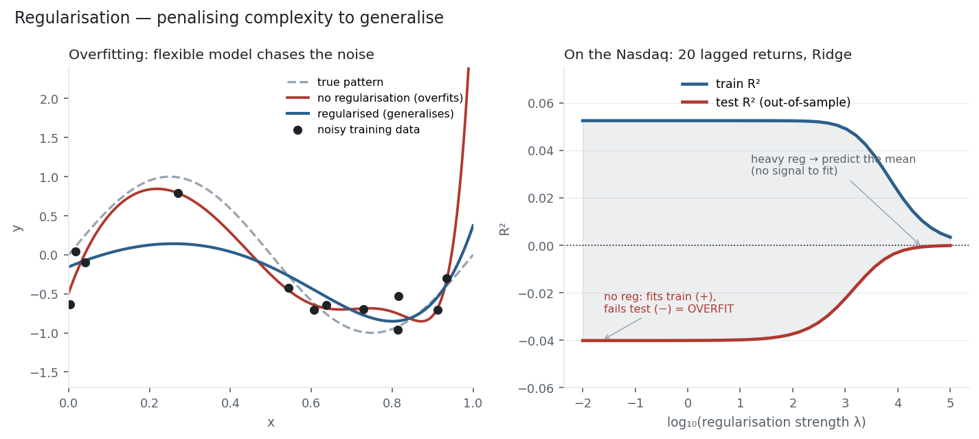
The honest reading is that here the optimal amount of regularisation is essentially “all of it.” That is not a failure of Ridge; it is Ridge correctly reporting what entropy, cross-entropy and information gain each reported in their own language — there is no reliable signal in these features, so the model that generalises best is the one that leans hardest on simplicity. In a domain where overfitting masquerades as skill, a method that defaults to humility and makes you pay for every parameter is not a constraint. It is the whole point.
Same multi_daily.csv as the previous entries (yfinance, adjusted closes). The market panel is a scikit-learn Ridge on 20 lagged NDX returns, 70/30 time-ordered split, features standardised; R^2 is relative to predicting the training mean. The left panel is an illustrative degree-11 fit to a noisy sine. Every number was checked.
Common mistakes
- Choosing λ on the training set. Training loss only rises with \lambda, so it can’t pick the sweet spot; tune on validation or cross-validation.
- Not scaling features. L1/L2 penalise raw coefficients, so features on larger scales are under-penalised; standardise first.
- Penalising the intercept. The bias term is usually left out of the penalty — shrinking it just biases predictions toward zero.
- Thinking more is always safer. Too much \lambda underfits (high bias); the goal is the minimum of validation error, not the maximum \lambda.
- Treating it as only L1/L2. Early stopping, dropout, data augmentation, and tree pruning are all regularisation — anything that trades fit for simplicity.
- Expecting it to create signal. Regularisation controls overfitting; it can’t manufacture predictability that isn’t there (as the Nasdaq result shows).