Mean Squared Error (MSE)
The default regression loss — average squared error, and why it fears outliers
Mean squared error is the loss the last two entries were quietly minimising — the parabola in the cost-function bowl and the surface gradient descent rolled down are both MSE. It is the default way to score a regression: average the squared misses. That squaring is the whole personality of MSE — it makes the loss smooth and easy to optimise, ties it directly to variance, and gives it a deep fear of outliers that matters enormously on fat-tailed markets.
The equation
\text{MSE} = \frac{1}{n}\sum_{i=1}^{n}(y_i - \hat y_i)^2, \qquad \text{RMSE} = \sqrt{\text{MSE}}
The mean of the squared residuals; RMSE is its square root, back in the original units.
What each symbol means
| Symbol | Meaning |
|---|---|
| MSE | mean squared error |
| RMSE | root mean squared error — same units as y |
| y_i | the true value |
| \hat y_i | the predicted value |
| y_i - \hat y_i | the residual (error) on example i |
| n | the number of examples |
Plain-English explanation
MSE scores a set of predictions by how far they miss, on average, after squaring each miss. Squaring does two things: it makes every error positive (so overshoots and undershoots don’t cancel), and it makes big misses count far more than small ones — an error of 3 contributes 9, an error of 1 contributes 1, so one big miss outweighs nine small ones. The average of those squared misses is the MSE; take its square root and you get the RMSE, which is back in the units of the thing you’re predicting and reads like a “typical error.”
That quadratic weighting is MSE’s defining trait, for better and worse. Its virtue: the squared-error curve is a smooth parabola with a simple slope everywhere, so gradient descent glides down it — the gradient of (y-\hat y)^2 is just -2(y-\hat y), a clean linear signal. Its vice: it is dominated by outliers. The robust alternative, mean absolute error (MAE), uses |y-\hat y| instead — the V-shaped curve in the figure — and barely reacts to extreme misses. The choice between them is a choice about what a “typical” error should mean: MSE says a few huge misses are unacceptable; MAE says every miss counts the same.
Why it matters in markets
MSE is the default regression loss, and on markets its outlier obsession is the thing to watch. Returns are fat-tailed (the kurtosis entry), so a handful of crash days carry enormous squared errors — and MSE weights them accordingly. On eleven years of Nasdaq returns, the worst 5% of days account for 47% of the total squared error but only 21% of the absolute error: fit a model under MSE and you are, whether you meant to or not, optimising mostly for those few extreme days. That is a feature if catastrophic misses are what you care about (risk models, options), and a bug if those days are noise you’d rather not chase — a median-like MAE fit is steadier.
MSE also carries the statistics of the whole library inside it. The MSE of a constant prediction is exactly the variance — and the constant that minimises it is the mean (MAE’s minimiser is the median). The R^2 that grades a regression is 1 - \text{MSE}/\text{Var}(y), the fraction of variance the model removes. And minimising MSE is equivalent to maximum-likelihood estimation under Gaussian noise — which is why least-squares regression and the normal distribution are joined at the hip, and why MSE is the “natural” loss whenever errors are assumed bell-shaped.
A simple worked example
Four predictions miss by e = [2, -1, 0, 3]. Square them: [4, 1, 0, 9], sum 14, divide by 4 → MSE = 3.5. The RMSE is \sqrt{3.5} = 1.87 — a “typical” miss of about 1.9. Compare the MAE: the average of [2, 1, 0, 3] is 1.5. The two disagree because of the 3: it contributes 9 of the 14 squared units (64% of the MSE) but only 3 of the 6 absolute units (50% of the MAE). One outlier moved the MSE far more than the MAE — the whole story of squared error in one row.
Python implementation
import numpy as np

def mse(y, y_hat):  return np.mean((y - y_hat) ** 2)
def rmse(y, y_hat): return np.sqrt(mse(y, y_hat))

# (sklearn: from sklearn.metrics import mean_squared_error)
y_hat = alpha + beta * x                    # AAPL predicted from NDX
print(round(mse(y, y_hat), 3))              # -> 1.278   (RMSE 1.13%/day, R^2 0.61)
The gradient of the squared error with respect to the prediction is -2 * (y - y_hat) — the clean linear signal gradient descent follows, and the reason MSE is the default loss to pair with it.
Manual / Excel calculation
| Task | Formula |
|---|---|
| squared error per row | =(A2-B2)^2 |
| MSE | =AVERAGE( the squared-error column ) |
| RMSE | =SQRT( MSE cell ) |
| MAE (robust cousin) | =AVERAGE(ABS(A2:A100 - B2:B100)) |
Excel’s =SUMXMY2(actual, predicted)/COUNT(actual) computes MSE in a single call.
Financial-market example — Nasdaq 100
Score the AAPL-from-NDX model this section keeps using. Its residuals have MSE = 1.28 (%²/day), so RMSE = 1.13% — a typical daily miss of just over one percent. Dividing out the variance gives R^2 = 1 - \text{MSE}/\text{Var} = 0.61: the Nasdaq return explains 61% of Apple’s daily variance, and the remaining 39% is Apple-specific. Same number three ways — it also equals the 0.78 correlation squared — so MSE, R^2, and correlation are one idea in different clothes.
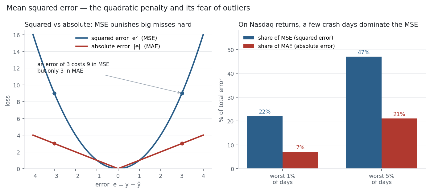
The fat-tail warning is the right panel. Predicting NDX returns with their mean, the squared errors are wildly concentrated: the worst 1% of days carry 22% of the total MSE, the worst 5% carry 47% — versus 7% and 21% of the MAE. The RMSE (1.39%) sits 45% above the MAE (0.96%), where a normal distribution would put it only 25% above; that gap is the fat tail showing up in the loss itself. So on markets, choosing MSE is choosing to let the crashes dominate what your model learns. Sometimes that is exactly right — just know that you are doing it.
Same multi_daily.csv as the previous entries (yfinance, adjusted closes). MSE, RMSE and R² are computed on the AAPL-on-NDX regression and on NDX returns; the concentration figures are the share of total squared vs absolute error from the most extreme days. Every number was checked.
Common mistakes
- Reading MSE in the wrong units. MSE is in squared units; report RMSE (same units as the target) to interpret it, and never compare raw MSE across differently-scaled targets.
- Forgetting MSE’s outlier sensitivity. A few extreme errors can dominate the score; on fat-tailed data check MAE too, or use a robust loss (Huber).
- Confusing the minimisers. MSE is minimised by the mean, MAE by the median — they give different fits when the data is skewed.
- Comparing an RMSE to nothing. RMSE is only meaningful against a baseline (the target’s own std, or a naive model); R^2 = 1 - \text{MSE}/\text{Var} does that normalisation.
- Using MSE for classification. For probabilities, cross-entropy (next up) is the right loss; MSE trains slowly and poorly there.
- Chasing a low training MSE. As with any loss, low MSE on the training set can be overfitting — judge it on held-out data.