Moving Averages (SMA & EMA)
Smoothing price into trend — equal weights vs recent-weighted, and the lag you pay for it
Price is noisy; trend is what you actually want to see. A moving average is the simplest way to extract it — average the last few prices and the day-to-day jitter cancels, leaving the drift. There are two flavours: the simple moving average weights every day in its window equally, and the exponential moving average fades older days out geometrically so recent prices count more. They are the workhorses of technical trading and the first building block of the models later in this section — but, as autocorrelation warned, smoothing a near-random walk produces signals weaker than they look.
The equation
The simple moving average is the mean of the last k prices; the exponential moving average is a recursive, weighted update:
\text{SMA}_t = \frac{1}{k}\sum_{i=0}^{k-1} P_{t-i} \qquad \text{EMA}_t = \alpha P_t + (1-\alpha)\,\text{EMA}_{t-1}, \quad \alpha = \frac{2}{k+1}
The SMA gives each of the last k prices weight 1/k; the EMA gives today weight \alpha and decays every older day by a factor (1-\alpha).
What each symbol means
| Symbol | Meaning |
|---|---|
| \text{SMA}_t | simple moving average at time t |
| \text{EMA}_t | exponential moving average at time t |
| P_t | the price at time t |
| k | the window length (the “period”) |
| \alpha | the EMA smoothing factor, 2/(k+1) — the weight on the newest price |
| 1-\alpha | the decay applied to the running average each step |
A larger k (smaller \alpha) means more smoothing and more lag; a smaller k hugs price but stays noisy.
Plain-English explanation
Prices wobble; a moving average smooths the wobble to show where price is heading. The simple moving average just takes the mean of the last k closes — a 50-day SMA is the average of the last 50 days, redrawn daily. Because every day in the window counts equally and the window is a hard cutoff, the SMA lags: it is centred on price about k/2 days ago, so it turns well after price does.
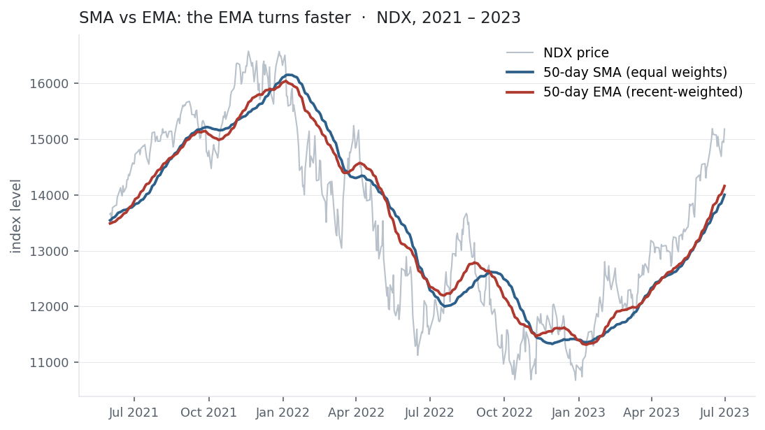
The exponential moving average trims the lag by weighting recent prices more. Each day it nudges the previous average a fraction \alpha of the way towards today’s price. Older prices never fully vanish — they fade geometrically — so the EMA has an infinitely long but rapidly shrinking memory. It reacts faster to turns (the figure), at the cost of a slightly bumpier line. The choice is always the same trade-off: smoother and slower (long SMA), or responsive and jumpier (short EMA).
Why it matters in markets
Moving averages are everywhere in trading: as trend filters (“only go long above the 200-day”), as support and resistance, and above all in crossovers — when a fast MA crosses a slow one, the “golden cross” (50 above 200) and “death cross” flag trend changes. They are also the smoothing kernel inside AR and ARIMA models, and the EMA’s recursive form is exactly the update rule reused in GARCH volatility and in the momentum term of ML optimisers.
But there is a catch this library keeps returning to. A moving average can only profit from trend — persistent, positive autocorrelation — and returns have almost none. So MA-crossover strategies look compelling on a chart and disappoint in a backtest. The honest test is below: on the Nasdaq, a classic 50/200 crossover did not beat buy-and-hold; it merely traded return for a smaller drawdown. A moving average describes the past — it does not predict the future.
A simple worked example
Five prices: [10, 12, 11, 13, 14]. The 3-day SMA on the last day is (11 + 13 + 14)/3 = 12.67. The 3-day EMA uses \alpha = 2/(3+1) = 0.5; starting from 10 it updates 10 \to 11 \to 11 \to 12 \to 13. On the final day the EMA reads 13 against the SMA’s 12.67 — pulled higher because it weights the recent jump to 14 more heavily. Same data, but the EMA leans towards the present.
Python implementation
import pandas as pd

px = pd.read_csv("../multi_daily.csv", index_col="Date", parse_dates=True)["NDX"]

sma50 = px.rolling(50).mean()                     # simple: equal weights
ema50 = px.ewm(span=50, adjust=False).mean()      # exponential: alpha = 2/(50+1)
print(round(2/(50+1), 4))                         # -> 0.0392   the smoothing factor

# a 50/200 crossover signal (long when the fast SMA is above the slow)
signal = (px.rolling(50).mean() > px.rolling(200).mean()).astype(int)
strat  = signal.shift(1) * px.pct_change()        # shift(1) avoids look-ahead bias
ewm(span=k) uses \alpha = 2/(k+1); adjust=False gives the recursive form above. The shift(1) is the most important line — trading today on today’s close is look-ahead bias.
Manual / Excel calculation
| Task | Formula |
|---|---|
| Simple moving average | =AVERAGE(B2:B51) (fill down for a 50-period SMA) |
| EMA smoothing factor | =2/(k+1) |
| EMA (recursive) | =α*B2 + (1-α)*[previous EMA cell] |
The first EMA cell is usually seeded with the SMA, and the recursion takes over from there.
Financial-market example — Nasdaq 100
The figure shows NDX through its 2021 top and 2022 fall with a 50-day SMA and a 50-day EMA. Both smooth the noise, but the EMA turns sooner at the top and the bottom — it weights the latest prices more, so it lags less (for a slightly bumpier line). A 50-day average sits about 24 days behind price; that lag is unavoidable, and it is why a moving average always confirms a trend rather than predicting it.
Does trading it pay? A textbook 50/200 crossover — hold NDX when the 50-day SMA is above the 200-day, sit in cash otherwise — over the full history:
| Strategy | CAGR | Sharpe | max drawdown |
|---|---|---|---|
| Buy and hold | 18.2% | 0.87 | −35.6% |
| 50/200 crossover | 15.4% | 0.86 | −28.0% |
The crossover (13 trades, invested 76% of the time) shaved the worst drawdown from −36% to −28% — but gave up nearly three points of annual return to do it, landing at essentially the same Sharpe. It did not beat holding; it swapped some upside for a smoother ride. That is the typical verdict for trend-following a market with little return autocorrelation: useful for shaping risk, not for manufacturing an edge.
Same multi_daily.csv as the previous entries (yfinance, adjusted closes). Code blocks are illustrative — every figure was computed and checked against that file.
Common mistakes
- Expecting crossovers to beat buy-and-hold. On weakly-autocorrelated markets they usually don’t; they reshape the risk profile, not the edge.
- Look-ahead bias. Trading on the same bar’s close that formed the signal inflates every backtest — lag the signal by one period.
- Forgetting the lag. A k-period MA is centred ~k/2 periods back; it confirms trends late, so its signals always trail the move.
- Over-optimising the windows. 50/200 “works” in hindsight; searching thousands of window pairs for the best backtest is textbook overfitting.
- Treating SMA and EMA as interchangeable. Same period, different behaviour — the EMA reacts faster and is noisier; choose for the job.
- Modelling on raw non-stationary prices. Fine for a visual trend, but AR/ARIMA want returns or a differenced, stationary series (entries to come).