Simple, Log & Cumulative Returns
Turning prices into returns — the two conventions, and how to chain them over time
Everything else in this library is built on returns, so it is worth being precise about what a “return” even is. Three of them come up constantly: the simple return (the percentage change everyone means), the log return (the modeller’s choice, because it adds across time), and the cumulative return (the total over a whole period). They are close cousins — but knowing which to use, and where they diverge, prevents a surprising number of bugs.
The equation
Three definitions, all from the price P_t:
r_t = \frac{P_t}{P_{t-1}} - 1 \qquad\text{(simple)}
\ell_t = \ln\frac{P_t}{P_{t-1}} = \ln(1 + r_t) \qquad\text{(log)}
R_{0:n} = \prod_{t=1}^{n}(1 + r_t) - 1 = \frac{P_n}{P_0} - 1 \qquad\text{(cumulative)}
Simple is the percentage change; log is the natural log of the price ratio; cumulative compounds the single-period returns into one total.
What each symbol means
| Symbol | Meaning |
|---|---|
| P_t | the price at time t |
| r_t | the simple return over period t |
| \ell_t | the log (continuously compounded) return over period t |
| R_{0:n} | the cumulative return from time 0 to n |
| \prod | product over the periods |
| \ln | natural logarithm |
Plain-English explanation
The simple return is what everyone means by “return”: the percentage change in price. Up 10% means r = 0.10. It is intuitive, and it is what you actually earn.
The log return is \ln(1+r) — the return under continuous compounding. For small moves it is almost identical to the simple return (a 1% day is 0.995% in logs), but it has one magic property: log returns add across time. The log return over a year is just the sum of the daily log returns. Simple returns don’t add — they compound.
The cumulative return is the total over a whole stretch: multiply all the (1+r_t) growth factors and subtract 1, which is the same as P_n/P_0 - 1. It is the equity-curve number — what a buy-and-hold investor actually made.
Why it matters in markets
The distinction that saves you: simple returns aggregate across assets, log returns aggregate across time. A portfolio’s simple return is the weighted average of its holdings’ simple returns (exactly), so simple returns are right for portfolio and cross-sectional work. A multi-period return is the sum of the log returns, so log returns are right for time-series modelling, annualising, and anything involving compounding. Reach for the wrong one and your portfolio maths or your time aggregation quietly breaks.
Two more reasons log returns dominate in modelling: they are roughly symmetric and unbounded below (a +50% move and the −33% that undoes it are +40.5% and −40.5% in logs — mirror images), and their summing to the total return makes the geometric mean and CAGR fall straight out (mean log return = \ln(1 + \text{geometric mean})). This is the same simple-vs-log fork flagged back in Mean Return, now made concrete.
A simple worked example
A stock goes 100 → 110 → 99 over two days.
- Simple: day 1 is 110/100 - 1 = +10\%; day 2 is 99/110 - 1 = -10\%.
- Cumulative: \tfrac{99}{100} - 1 = -1\% — not 10\% + (-10\%) = 0\%. You cannot add simple returns: a 10% gain then a 10% loss leaves you down 1%.
- Log: \ln(1.10) = +9.53\% and \ln(0.90) = -10.54\%, and these do add: 9.53\% - 10.54\% = -1.01\%, which is exactly \ln(99/100). Exponentiate and you are back at −1%.
Python implementation
import numpy as np
import pandas as pd

px = pd.read_csv("../multi_daily.csv", index_col="Date", parse_dates=True)["NDX"]

simple = px.pct_change()                          # P_t / P_{t-1} - 1
log_r  = np.log(px / px.shift(1))                 # ln(P_t / P_{t-1})
cumret = (1 + simple).prod() - 1                  # product of growth factors, minus 1

print(round(cumret * 100, 1))                     # -> 587.0   (%)  = P_end/P_0 - 1
print(round(log_r.sum(), 4))                      # -> 1.9271       sum of logs = ln(P_end/P_0)
print(round((np.exp(log_r.sum()) - 1) * 100, 1))  # -> 587.0   same cumulative, via logs
pct_change() gives simple returns; np.log(px/px.shift(1)) gives log returns; the cumulative return is (1+r).prod()-1, or equivalently exp(sum of logs) - 1.
Manual / Excel calculation
With prices in column B:
| Task | Formula |
|---|---|
| Simple return | =B3/B2 - 1 |
| Log return | =LN(B3/B2) |
| Cumulative return | =PRODUCT(1+returns) - 1 (or =EndPrice/StartPrice - 1) |
Never SUM simple returns to get a cumulative — that is the classic error. Sum the log returns, or take the product of the (1 + r) factors.
Financial-market example — Nasdaq 100
Over 2015–2026 NDX went from 4,230 to 29,061 — a cumulative (simple) return of 29{,}061 / 4{,}230 - 1 = 587\%. The daily log returns over that span sum to exactly 1.9271, which is \ln(29{,}061/4{,}230) — and e^{1.9271} - 1 = 587\% recovers the same total. That equality is the whole point of log returns: the messy product of ~2,900 daily growth factors collapses into a single sum.
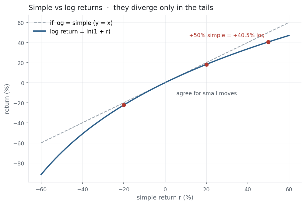
On any single day the two are almost indistinguishable — a −0.32% simple day is a −0.32% log day. They part company only in the tails: a +50% move is +40.5% in logs, a −50% move is −69.3%. That asymmetry — a −100% simple return is -\infty in logs — is exactly why log returns are the natural coordinate for modelling extremes.
Same multi_daily.csv as the previous entries (yfinance, adjusted closes). Code blocks are illustrative — every figure was computed and checked against that file.
Common mistakes
- Adding simple returns across time. +10% then −10% is −1%, not 0%. Compound them (product of 1+r), or use log returns, which do add.
- Averaging log returns across assets. A portfolio’s return is the weighted average of the simple returns, not the log returns. Use simple for cross-sectional work.
- Treating log and simple as interchangeable. Fine for a single small day; wrong for big moves or long horizons, where the gap compounds.
- Mixing conventions in one calculation. A mean or Sharpe on log returns isn’t directly comparable to one on simple returns — pick one and stay with it.
- Thinking cumulative return is a sum. The equity curve is
(1+r).cumprod(), never a running sum of returns. - Forgetting the −100% floor. A simple return can’t fall below −100%; a log return can go to -\infty — realistic for continuous modelling, but not for a bounded P&L.