The Sigmoid Function
Turning any score into a probability — the S-curve behind logistic regression
The regression entries predicted a number; classification predicts a probability — and the sigmoid is the function that makes the leap. A model produces a raw score, any real number from -\infty to +\infty, and the sigmoid squashes it into the interval (0, 1) so it can be read as “the probability this belongs to class 1.” It is the activation at the heart of logistic regression, the output neuron of every binary classifier, and — through a remarkably clean derivative — a building block of the training that runs neural networks.
The equation
\sigma(z) = \frac{1}{1 + e^{-z}}, \qquad \sigma(z) \in (0, 1)
Its inverse is the logit (the log-odds), z = \ln\frac{p}{1-p}, and its derivative is unusually clean: \sigma'(z) = \sigma(z)\,(1 - \sigma(z)).
What each symbol means
| Symbol | Meaning |
|---|---|
| \sigma(z) | the sigmoid (logistic) function, output in (0,1) |
| z | the input — a raw score, or log-odds |
| e | Euler’s number, \approx 2.718 |
| \sigma'(z) | the derivative, \sigma(z)(1-\sigma(z)) |
| logit | the inverse, \ln\frac{p}{1-p} — the log-odds |
Plain-English explanation
The sigmoid takes any number and bends it into a probability. Feed it 0 and it returns 0.5; feed it a large positive number and it returns something just under 1; a large negative number and it returns just over 0. In between it traces a smooth S — rising fastest around zero and flattening at both ends. That shape is exactly what you want to convert a model’s raw score, which can be anything, into a “probability of yes.”
Read the input as log-odds and the sigmoid becomes an accounting identity. A score of 0 means even odds (0.5); a score of 2 means log-odds of 2 — odds of about 7-to-1, a probability of 0.88; a score of −2 flips that to 0.12. The inverse map z = \ln\frac{p}{1-p} is the logit, and it is why logistic regression works: it fits a straight line in log-odds space, and the sigmoid folds that line back into probabilities. The other special feature is the derivative, \sigma(1-\sigma): the slope can be written using only the function’s own output, which makes it cheap to use in gradient-based training. That slope peaks at 0.25 in the middle and falls to nearly zero in the flat tails — the vanishing gradient that makes deep sigmoid networks hard to train and pushed hidden layers toward ReLU.
Why it matters in markets
The sigmoid is where a model stops asserting and starts hedging, which is exactly the posture markets demand. A regression that outputs “tomorrow’s return is +0.3%” is brittle; a classifier that outputs “P(up tomorrow) = 0.57” is honest about the uncertainty, and the sigmoid is what produces that number. It is the entire output stage of logistic regression — p = \sigma(w \cdot x + b) — and of every binary neural classifier: whatever features go in, a linear score comes out, and the sigmoid turns it into a probability with a natural decision boundary at 0.5 (where the score is 0).
Its quirks matter in practice. Because it saturates, a confident wrong prediction sits in a flat region where the gradient nearly vanishes, so the model learns slowly from its worst mistakes — a problem the cross-entropy loss (the next entry) is specifically designed to cancel. And because it is bounded, it can never output exactly 0 or 1, which is sensible: no model should be infinitely certain. Its shape is close to the normal CDF that the probit model uses — the two give near-identical probabilities — and the sigmoid wins on sheer analytic convenience.
A simple worked example
Take a raw score of z = 2. Then e^{-2} = 0.135, so \sigma(2) = 1/(1 + 0.135) = 0.881 — the model assigns an 88% probability to class 1. Check it in log-odds: a probability of 0.88 means odds of 0.88/0.12 \approx 7.3, and \ln(7.3) = 1.99 \approx 2, recovering the score. A score of 0 gives 0.5 (even odds); doubling the score to 4 pushes the probability to 0.98 but only adds 0.10 — the S-curve is already flattening, so extra confidence in the score buys less and less probability.
Python implementation
import numpy as np

def sigmoid(z):
    return 1 / (1 + np.exp(-z))

p     = sigmoid(2.0)             # -> 0.881
logit = np.log(p / (1 - p))     # -> 2.0    (the inverse: log-odds)

# logistic regression = a linear score fed through the sigmoid:
prob_up = sigmoid(w @ x + b)    # P(class 1)
For large negative z, np.exp(-z) overflows; production code uses a numerically stable form (scipy.special.expit) that handles both tails.
Manual / Excel calculation
The sigmoid is one cell: =1/(1+EXP(-z)). The log-odds inverse is =LN(p/(1-p)). To sanity-check a value, remember three anchors — \sigma(0)=0.5, \sigma(\pm 2)\approx 0.88/0.12, \sigma(\pm 4)\approx 0.98/0.02 — and that the curve is symmetric about (0,\ 0.5), i.e. \sigma(-z) = 1 - \sigma(z).
Financial-market example — Nasdaq 100
Turn the sigmoid loose on a real classification: predict whether the Nasdaq rises tomorrow from today’s return. Fit a logistic regression and it becomes P(\text{up tomorrow}) = \sigma(-0.046\cdot\text{today} + 0.245). Two things are worth reading off it. The intercept encodes the base rate — 56% of next-days were up over this stretch, the market’s upward drift — so with no information the model already leans bullish. The slope is negative, and that is the −0.12 mean-reversion this whole library keeps meeting, now wearing a probability: a down day today raises tomorrow’s up-probability, an up day lowers it.
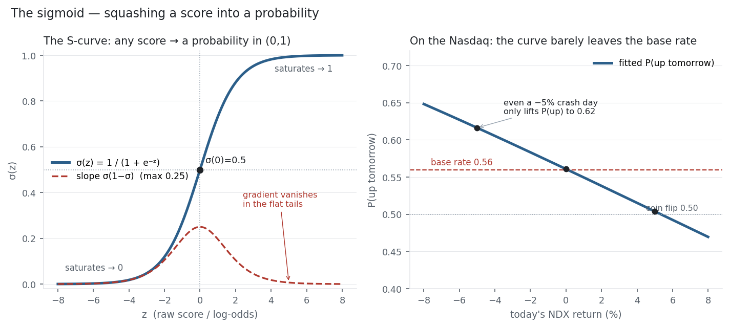
But look how little the score moves the output (right panel). Even a −5% crash day only lifts P(up) to 0.62, and a +5% day only drops it to 0.50; across every day in eleven years the probability stays inside 0.42 to 0.69, hugging the 0.56 base rate. The sigmoid is doing its job perfectly — it is a faithful, well-behaved probability machine — but it can only pass along the signal in the score, and for near-random returns that signal is faint. This is the honest shape of the efficient market in classification terms: you can produce a genuine probability, it just sits stubbornly close to the base rate.
Same multi_daily.csv as the previous entries (yfinance, adjusted closes). The logistic regression predicts P(next-day NDX return > 0) from the current day’s return (scikit-learn); the base rate and coefficients are computed from the data. Every number was checked.
Common mistakes
- Reading the output as certainty, not probability. \sigma = 0.9 means 90% odds, not “yes”; calibrate and threshold deliberately (0.5 is a default, not a law).
- Using sigmoid for multi-class problems. For more than two classes you need softmax (next entry); a pile of independent sigmoids won’t give probabilities that sum to 1.
- Sigmoid hidden layers in deep nets. Saturation kills gradients in deep stacks; use ReLU for hidden layers and reserve sigmoid for a binary output.
- Pairing it with squared-error loss. MSE + sigmoid gives a slow, non-convex objective; cross-entropy is built to cancel the sigmoid’s saturating gradient.
- Forgetting numerical overflow. Naive
1/(1+exp(-z))overflows for large |z|; use a stable implementation. - Confusing the score with the probability. The linear part w\cdot x + b lives on the log-odds scale; only after the sigmoid is it a probability.