Z-score & the Normal Distribution

Standardising a value, the bell curve it lives on — and why returns refuse to fit it

The z-score (how many standard deviations from the mean) and the normal distribution it maps onto: the 68-95-99.7 rule, the central limit theorem, and the fat-tailed reality that breaks the Gaussian assumption in markets.

A great deal of this library leans on one distribution: the normal. Gaussian VaR, the interpretation of a Sharpe ratio, confidence intervals — all assume the bell curve. The z-score is how you speak to it: it re-expresses any value as “how many standard deviations from the mean,” so you can look up how unusual it is. Together they are the backbone of statistical reasoning — and, in markets, a persistent source of overconfidence, because returns are fatter-tailed than the bell curve allows.

The equation

The z-score standardises a value; the normal distribution is the bell curve it maps onto:

z = \frac{x - \mu}{\sigma} \qquad f(x) = \frac{1}{\sigma\sqrt{2\pi}}\,e^{-\frac{1}{2}\left(\frac{x-\mu}{\sigma}\right)^2}

The z-score measures distance from the mean in standard-deviation units; the normal density f(x) is fully determined by just \mu and \sigma.

What each symbol means

Symbol	Meaning
z	the z-score — number of standard deviations from the mean
x	the value being standardised
\mu	the mean
\sigma	the standard deviation
f(x)	the normal probability density at x
e,\ \pi	the usual constants (≈2.718, ≈3.142)

A z of 0 sits at the mean; z = +2 is two σ above it. Standardising any normal gives the standard normal: \mu = 0, \sigma = 1.

Plain-English explanation

The z-score answers how unusual is this? Subtract the mean, divide by the standard deviation, and any number becomes a count of standard deviations. A test score, a daily return, and a person’s height all become comparable once they are z-scores — a z of 2 is equally rare in each, if each is normal.

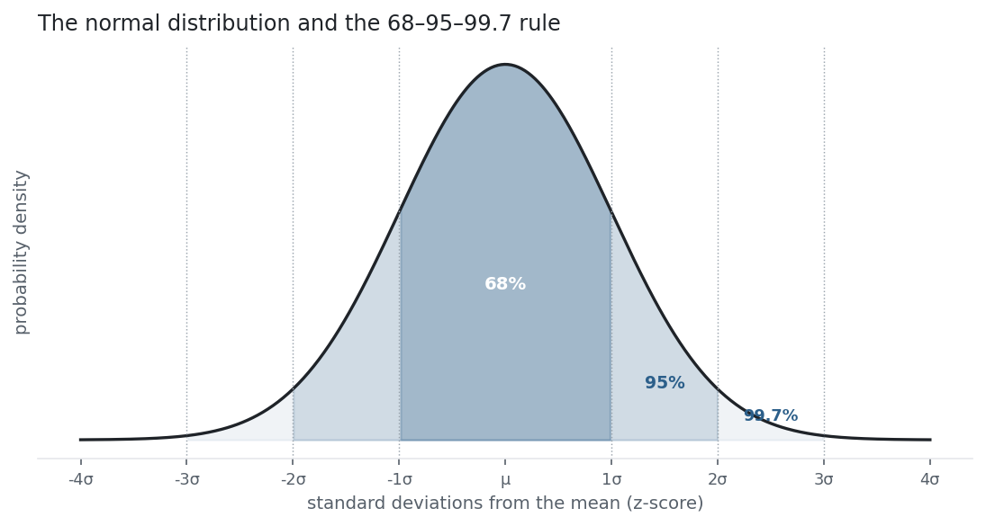
The normal distribution is the bell curve those z-scores fall on. It is the most important distribution in statistics for two reasons: it is fully described by just its mean and standard deviation, and — via the central limit theorem — sums of many small independent effects drift towards it, which is why it appears everywhere. Its signature is the 68-95-99.7 rule: about 68% of observations land within ±1σ of the mean, 95% within ±2σ, and 99.7% within ±3σ (the figure). A z beyond ±3 should be genuinely rare.

Why it matters in markets

The normal is the default assumption baked into a huge amount of finance: parametric VaR uses z = 1.645 for its 95% loss, option pricing assumes log-normal prices, and the whole language of “a 3-sigma move” treats σ as if the world were Gaussian. The z-score is the currency of that world — it turns a raw return into a probability through the normal’s tables.

The catch, and the reason this entry carries a warning, is that returns are not normal. Skewness and kurtosis already showed the tails are fat; z-scores make it visceral. Under a normal a −4σ day is roughly a once-in-a-lifetime event, yet markets produce them every few years. When a risk model quietly assumes normality, it prices those disasters as essentially impossible — which is precisely how “impossible” losses keep arriving. The normal is an indispensable baseline and a treacherous literal model.

A simple worked example

NDX rises 3% on a day. With a mean daily return of 0.12% and a daily σ of 1.15%:

z = \frac{3\% - 0.12\%}{1.15\%} = 2.5.

A 2.5σ day. Under a normal, the chance of a move that large or larger is about 0.6% — roughly 1 trading day in 160. The z-score turned “up 3%” into “a 1-in-160 event,” which is exactly what makes it useful.

Python implementation

import pandas as pd
from math import erf, sqrt

r = (pd.read_csv("../multi_daily.csv", index_col="Date", parse_dates=True)["NDX"]
       .pct_change().loc["2025-07-01":"2026-06-30"].dropna())

z = (r - r.mean()) / r.std(ddof=1)          # standardise every day
print(round(z.min(), 2))                     # -> -4.26   the worst day, in sigmas

Phi = lambda x: 0.5 * (1 + erf(x / sqrt(2)))  # standard-normal CDF (= scipy.stats.norm.cdf)
print(round(1 / Phi(z.min())))               # -> 98753   1 in ~98,753 days, if normal

scipy.stats.norm.cdf / .ppf do the same lookups; the erf version is dependency-free.

Manual / Excel calculation

Task	Formula
z-score	=(x - AVERAGE(range)) / STDEV.S(range)
Normal probability below z	=NORM.S.DIST(z, TRUE)
Value for a given probability	=NORM.S.INV(p)

NORM.S.DIST and NORM.S.INV are the standard-normal CDF and its inverse — the lookup tables as functions.

Financial-market example — Nasdaq 100

Turn every NDX day of the year into a z-score and count how they fall:

Band	NDX	Normal
within ±1σ	72.5%	68.3%
within ±2σ	95.6%	95.4%
within ±3σ	99.2%	99.7%

The standard normal with the 68-95-99.7 bands. NDX is more peaked than this in the middle and fatter in the tails than it allows at the edges.

It looks like a near-match, and through the middle it is. But read the ±3σ row: a normal keeps 99.7% of days inside ±3σ, NDX only 99.2% — more days escaped beyond 3σ than the bell curve permits. The proof is the single worst day, a −4.77% drop: a z-score of −4.26. Under a normal, a day that bad or worse should appear about once every 98,753 trading days — nearly four centuries. NDX served one up inside a single year. The distribution is more peaked in the middle and far fatter in the tails than the normal — excess kurtosis made concrete. The z-score is still the right tool; the normal’s probability for it is simply wrong.

Same multi_daily.csv as the previous entries (yfinance, adjusted closes). Code blocks are illustrative — every figure was computed and checked against that file.

Common mistakes

• Assuming normality by default. Real returns are fat-tailed and skewed; the normal understates extremes badly. Use it as a baseline, not a truth.
• Reading a z-score as a normal probability. z is just a distance in σ units; converting it to a probability only works if the data really is normal.
• Standardising with the wrong σ. Sample vs population (n vs n-1) changes the z, and a σ estimated from few points is itself uncertain.
• Treating “3-sigma” as impossible. Under fat tails, 3σ+ events are many times more common than 0.3%; risk limits built on the normal get breached routinely.
• Forgetting the mean. A z-score is distance from the mean, not from zero — with a non-zero drift they differ.
• Confusing the standard normal with any normal. Only after standardising do the 1.645 / 1.96 / 2.576 lookup values apply.