Sortino Ratio
Sharpe, but only the downside counts — reward per unit of harmful risk
The Sharpe ratio has one awkward feature: it treats a big up-day as “risk,” penalising the volatility you actually want. The Sortino ratio fixes that — it divides excess return not by total volatility but by downside deviation, the spread of only the returns that fell short of a target. It is the right tool whenever returns are asymmetric.
The equation
\text{Sortino} = \frac{\bar r - r_f}{\sigma_d}, \qquad \sigma_d = \sqrt{\frac{1}{n}\sum_{t=1}^{n}\min\!\left(r_t - \tau,\; 0\right)^2}
Same numerator as Sharpe — excess return — but the denominator is the downside deviation \sigma_d: take each return’s shortfall below a target \tau (returns above target contribute zero), square it, average over all n periods, and root.
What each symbol means
| Symbol | Meaning |
|---|---|
| \text{Sortino} | reward per unit of downside risk |
| \bar r - r_f | excess return (the same numerator as Sharpe) |
| \sigma_d | downside deviation — the “harmful” volatility only |
| \tau | the target / minimum acceptable return (MAR); usually 0 or r_f |
| \min(r_t - \tau,\,0) | the shortfall — negative below target, zero above |
| n | number of periods — all of them, not just the losing ones |
The detail that trips people up is that n: you divide by the total number of periods, not the count of losing days. Dividing by only the losers is a different, non-standard statistic.
Plain-English explanation
Standard deviation counts a +5% day and a −5% day as equally “risky,” even though only one of them hurts. The Sortino ratio keeps everything else the same but measures risk with downside deviation: it looks only at returns below your target (usually zero, or the risk-free rate), squares those shortfalls, and averages. Upside volatility is simply ignored.
So an asset that jumps around but mostly upward is rewarded, while one that grinds down is punished. Because downside deviation is always smaller than total volatility, a profitable asset’s Sortino is always higher than its Sharpe — and the interesting information is in how much higher.
Why it matters in markets
Sortino matters most exactly where Sharpe is weakest: asymmetric returns. For a positively skewed strategy — small frequent losses, occasional big wins (trend-following, long options) — Sharpe unfairly penalises the upside spikes that are the whole point; Sortino doesn’t. For a negatively skewed one — steady gains, rare crashes (selling options, carry) — a Sortino that stays high while the return stream quietly builds tail risk is a cue to go look at drawdown and kurtosis.
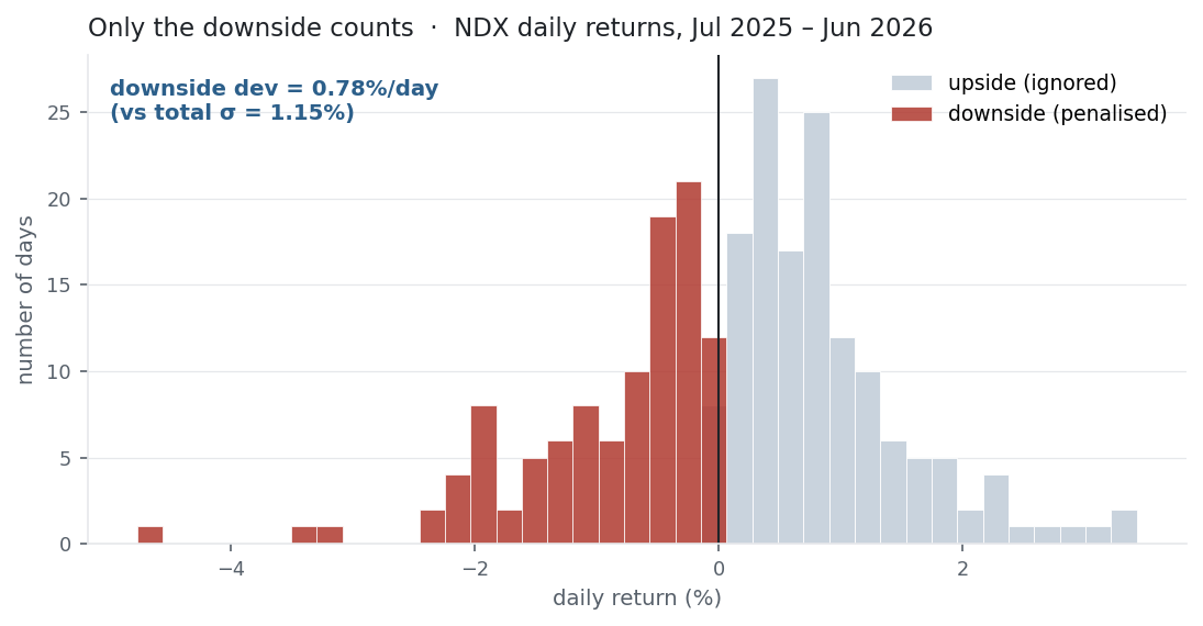
In practice allocators quote both: Sharpe for the overall risk-adjusted picture, Sortino for whether the risk being penalised is the risk that actually matters. The gap between them is a quick read on the shape of the returns.
A simple worked example
The running set [+2\%, -1\%, +3\%] has only one losing return. With target \tau = 0, the downside deviation uses just that −1% — the other two contribute zero — divided across all three periods:
\sigma_d = \sqrt{\tfrac{1}{3}\left(0^2 + (-0.01)^2 + 0^2\right)} = \sqrt{\tfrac{0.0001}{3}} = 0.58\%.
So \text{Sortino} = 1.33\% / 0.58\% = 2.31 per period, against a Sharpe of 1.33\%/2.08\% = 0.64. Ignoring the two up-days shrinks the denominator sharply, and Sortino rewards the asset for having mostly gained.
Python implementation
import numpy as np
import pandas as pd

r = (pd.read_csv("../multi_daily.csv", index_col="Date", parse_dates=True)
       .pct_change().loc["2025-07-01":"2026-06-30"])["NDX"]

target   = 0.0                                    # MAR; use rf/252 for a risk-free target
downside = np.minimum(r - target, 0.0)            # shortfalls (0 when above target)
dd       = np.sqrt((downside**2).mean())          # downside deviation: divide by ALL n
sortino  = np.sqrt(252) * (r.mean() - target) / dd
print(round(sortino, 2))                           # -> 2.46

# Sharpe, for comparison
print(round(np.sqrt(252) * r.mean() / r.std(ddof=1), 2))   # -> 1.68
The trap is the denominator: (downside**2).mean() divides by the full sample. Dividing by (downside < 0).sum() instead — a common error — inflates the ratio and breaks comparability with anyone else’s Sortino.
Manual / Excel calculation
By hand: for each return take \min(r_t - \tau, 0); square it; average over all rows; square-root → downside deviation. Then (\bar r - r_f)/\sigma_d \times \sqrt{252}.
Excel has no built-in downside-deviation function, so build it. With returns in B2:B252 and shortfalls =MIN(B2-0,0) in C2:C252:
| Task | Formula |
|---|---|
| Downside deviation | =SQRT(SUMSQ(C2:C252)/COUNT(B2:B252)) |
| Annualised Sortino (rf 0) | =AVERAGE(B2:B252)/SQRT(SUMSQ(C2:C252)/COUNT(B2:B252))*SQRT(252) |
SUMSQ sums the squared shortfalls (up-days add zero), and dividing by COUNT of all rows keeps the correct n.
Financial-market example — Nasdaq 100
The same basket, target \tau = 0 and r_f = 0, Sharpe alongside Sortino (annualised), ranked by Sortino:
| Ticker | Sharpe | Sortino | Sortino / Sharpe |
|---|---|---|---|
| AAPL | 1.59 | 2.48 | 1.56 |
| NDX | 1.68 | 2.46 | 1.46 |
| NVDA | 0.85 | 1.26 | 1.48 |
| PEP | 0.40 | 0.63 | 1.57 |
| MSFT | −0.91 | −1.19 | 1.31 |
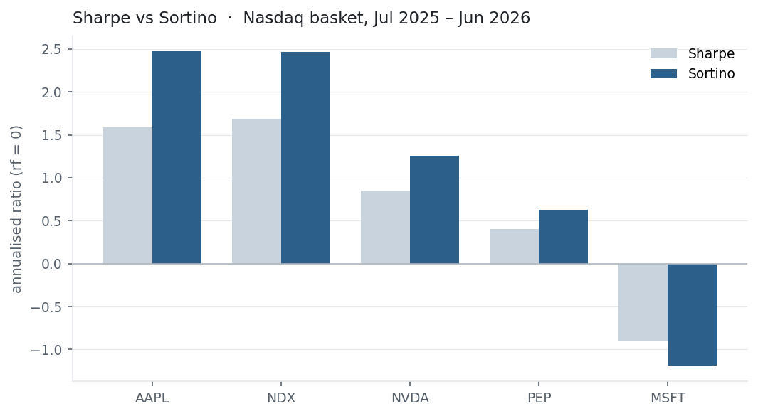
Every profitable name’s Sortino sits above its Sharpe, because downside deviation is smaller than total volatility (for NDX, 12.5% vs 18.2% annualised). But the size of the lift — and even the order — changes. On Sharpe the index leads (1.68 vs AAPL’s 1.59); on Sortino AAPL edges ahead (2.48 vs 2.46), because more of AAPL’s volatility is to the upside, exactly the volatility Sortino refuses to punish. MSFT is the mirror image: its Sortino (−1.19) is worse than its Sharpe (−0.91), because for a money-loser the damage is all downside. For the same returns, the two ratios can rank a book differently — and the difference is the shape of the risk.
Same multi_daily.csv as the previous entries (yfinance, adjusted closes). Code blocks are illustrative — every figure was computed and checked against that file.
Common mistakes
- Dividing by the number of losing periods. Standard downside deviation divides by the total n; using only the loss count changes the statistic and breaks comparability with published Sortinos.
- Not stating the target. \tau can be 0 or r_f; changing it changes which returns count as downside, and so the ratio. Always say which you used.
- Annualising with ×252. Downside deviation scales like σ (√time) — use \sqrt{252}.
- Treating a high Sortino as “safe.” It still says nothing about the size of the rare loss; pair it with maximum drawdown and kurtosis.
- Reading Sortino on Sharpe’s scale. A higher Sortino is expected (the denominator is smaller by construction), not impressive on its own — compare like with like.
- Bothering with it for symmetric returns. If skew ≈ 0, Sortino ≈ \sqrt{2}\times Sharpe and adds little; its value is entirely in asymmetric strategies.