t-statistic, p-value & Confidence Interval

Is the result real or noise? — the standard error, and the three numbers that decide

core statistics

inference

Statistical significance for a mean or a strategy: the standard error, the t-statistic, the p-value, and the confidence interval. Why the t-stat of a year’s return equals its Sharpe, and why proving an edge takes so long.

Author

David Maguire

Every backtest produces a number — a mean return, an alpha, a Sharpe. The only question that matters is whether it is a real edge or a lucky draw. Statistical inference answers it with three linked quantities: the t-statistic (how many standard errors your estimate sits from “no effect”), the p-value (the probability of a result this extreme by chance), and the confidence interval (the range of values the truth plausibly takes). All three rest on one humble number — the standard error — and together they are the immune system against fooling yourself.

The equation

The standard error of the mean, the t-statistic against a null \mu_0, and the 95% confidence interval:

\text{SE} = \frac{\sigma}{\sqrt{n}} \qquad t = \frac{\bar x - \mu_0}{\text{SE}} \qquad \text{CI}_{95\%} = \bar x \pm 1.96\,\text{SE}

The p-value is the tail probability beyond |t| — the chance of a t this large if the null were true.

What each symbol means

Symbol	Meaning
\text{SE}	standard error — the standard deviation of the estimate itself
\sigma	the sample standard deviation
n	the number of observations
\bar x	the sample mean (the estimate)
\mu_0	the null-hypothesis value — usually 0 (“no edge”)
t	the t-statistic — estimate over its standard error
1.96	the 95% two-sided value (from the normal; use the t-value for small n)

The standard error is the key: it shrinks like 1/\sqrt{n}, so more data sharpens every estimate — the statistical reason more history is always better.

Plain-English explanation

An average from data is only an estimate — a different sample would give a slightly different number. The standard error measures how much that estimate wobbles: \sigma/\sqrt{n}. It is the noise around your signal.

The t-statistic is signal-to-noise: how many standard errors your estimate sits above zero. A t of 2 means “two standard errors from no-effect” — the rough threshold for significance. The p-value turns that into a probability: p = 0.05 means a result this strong would occur 5% of the time even with no real effect; below 0.05, by convention, you call it significant. The confidence interval flips it around — instead of one number it gives a range, the band of true values consistent with your data. If the 95% CI excludes zero, the effect is significant; if it contains zero, you cannot rule out “nothing.”

Why it matters in markets

This is the machinery that separates a discovery from a fluke, and in quant finance the news is sobering. The t-statistic of a mean return is exactly the Sharpe ratio times the square root of the number of periods:

t = \frac{\bar r}{\sigma/\sqrt{n}} = \frac{\bar r}{\sigma}\sqrt{n} = \text{SR}_{\text{period}}\sqrt{n}.

Over one year of daily data that makes t equal to the annualised Sharpe. So a Sharpe of 2 gives a barely-significant t of 2 after a whole year; a Sharpe of 0.5 needs sixteen years to clear the bar (the figure). Most “edges” simply cannot be proven from the data available — which is why an out-of-sample t-stat matters more than a backtested return, and why testing thousands of strategies (as in the backtest-overfitting experiment) makes p-values almost meaningless: run 100 dead strategies and about 5 will look “significant” at p = 0.05 by pure chance. Significance is necessary, not sufficient — and far harder to earn than it looks.

A simple worked example

A strategy with 100 trades, average trade +0.5%, trade standard deviation 2%:

\text{SE} = \frac{2\%}{\sqrt{100}} = 0.2\%, \qquad t = \frac{0.5\%}{0.2\%} = 2.5.

A t of 2.5 gives a two-sided p-value of about 0.012 — below 0.05, so significant. The 95% confidence interval is 0.5\% \pm 1.96(0.2\%) = [0.11\%,\ 0.89\%], which excludes zero. The edge is real at the 5% level. Halve the sample to 25 trades and the SE doubles, t falls to 1.25, and the same edge is no longer significant — nothing changed but the evidence.

Python implementation

import numpy as np
import pandas as pd
from math import erf, sqrt

r = (pd.read_csv("../multi_daily.csv", index_col="Date", parse_dates=True)["NDX"]
       .pct_change().loc["2025-07-01":"2026-06-30"].dropna())

n  = len(r)
se = r.std(ddof=1) / np.sqrt(n)              # standard error of the mean
t  = r.mean() / se                           # t-stat against "mean = 0"
Phi = lambda x: 0.5 * (1 + erf(x / sqrt(2)))
p  = 2 * (1 - Phi(abs(t)))                    # two-sided p-value (normal approx, large n)
ci = (r.mean() - 1.96*se, r.mean() + 1.96*se)
print(round(t, 2), round(p, 3))              # -> 1.68  0.093   (NOT significant at 5%)
print([round(c*100, 3) for c in ci])         # -> [-0.02, 0.264]   the 95% CI contains 0

scipy.stats.ttest_1samp does this in one call using the exact t-distribution.

Manual / Excel calculation

Task	Formula
Standard error	`=STDEV.S(range)/SQRT(COUNT(range))`
t-statistic	`=AVERAGE(range)/(STDEV.S(range)/SQRT(COUNT(range)))`
p-value (two-sided)	`=T.DIST.2T(ABS(t), COUNT(range)-1)`
95% CI half-width	`=CONFIDENCE.T(0.05, STDEV.S(range), COUNT(range))`

Financial-market example — Nasdaq 100

NDX rose about 30% over the year — an annualised Sharpe of 1.68. Is its daily mean return statistically greater than zero? The daily mean was 0.122% with a standard error of 0.072% (σ = 1.15%, n = 251), so

t = \frac{0.122\%}{0.072\%} = 1.68, \qquad p = 0.093.

Not significant at the 5% level — and note t = 1.68 is exactly the annualised Sharpe. The 95% confidence interval for the daily mean is [-0.02\%,\ +0.26\%], which annualises to a staggering −5% to +66%: after a full year, the data cannot even rule out that NDX’s true expected return is negative.

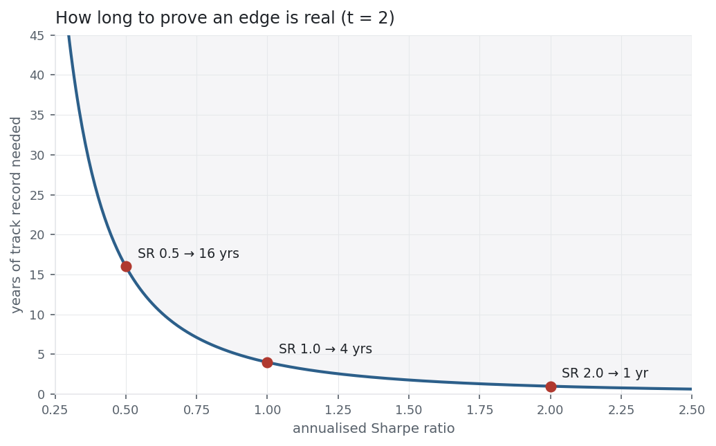
Curve of years-to-significance falling steeply as the annualised Sharpe rises — Years of track record a strategy needs before its Sharpe reaches t = 2. A Sharpe of 1 takes four years; a Sharpe of 0.5 takes sixteen.

That is not a quirk of this window; it is the rule. The figure shows how many years of track record a strategy needs before its Sharpe clears t = 2: a Sharpe of 1 takes four years, a Sharpe of 0.5 takes sixteen. Returns are so noisy that even a genuinely good strategy spends years indistinguishable from luck — the single strongest reason to distrust a short, glossy backtest.

Same multi_daily.csv as the previous entries (yfinance, adjusted closes). Code blocks are illustrative — every figure was computed and checked against that file.

Common mistakes

Reading p < 0.05 as “probably true.” It is the chance of the data under the null, not the chance the effect is real — and 0.05 is an arbitrary convention.
Ignoring multiple testing. Test many strategies and some clear p = 0.05 by chance; the more you try, the less any single “significant” result means.
Forgetting SE shrinks like √n. Quadruple the data to halve the standard error — significance is bought with sample size, and short samples prove little.
Confusing statistical and economic significance. A tiny edge can be statistically significant with enough data yet worthless after costs.
Treating the CI as “95% chance the truth is in here.” Strictly it is a statement about the procedure over repeated samples; what matters practically is whether it contains zero.
Using the normal for small n. For few observations use the t-distribution (fatter tails); and returns’ own fat tails make even the t optimistic.