Bayesian Change-Point Detection
Detecting a regime shift the day it happens — the run-length posterior, and a real-time alarm for the market’s turning points
The regime-aware modelling entry fit a hidden Markov model to split the Nasdaq’s history into calm and turbulent states, and the whole decision-systems tier has run on the regime environment that HMM defined. But that HMM is fit on the entire history at once — it is a smoother, and its regime labels use data from the future of every point it labels. That is hindsight, and hindsight cannot trade. A live system needs the opposite: to know a regime has changed as soon as possible after it happens, using only data up to today. That is change-point detection, and Bayesian Online Change-Point Detection (BOCPD, Adams–MacKay 2007) is its canonical form — a filter that updates a posterior over how long the current regime has lasted on every new observation, and raises an alarm the moment that posterior collapses. It is the real-time detection layer the proposal’s Regime Agent needs alongside the HMM: the HMM says “these were the regimes”; BOCPD says “a regime just changed, today.”
1. What problem does it solve?
Online detection of a structural break — a change in the data-generating distribution — with the shortest possible delay and using only past data. The offline question (“where, in this completed history, were the regimes?”) is what the HMM answers; it is easier, because it can look forward. The online question (“has the regime changed as of now?”) is what a trading system actually faces, and it is strictly harder: at the moment a crash begins there is almost no data confirming it yet. BOCPD gives a principled, probabilistic answer that sharpens with each new observation, so a system can de-risk early into a developing shift rather than after the drawdown has already happened.
2. The run-length posterior
BOCPD’s idea is to track a single latent quantity: the run length r_t, the number of steps since the last change-point. If r_t is large the current regime is well-established; when a change occurs r_t drops to 0 and starts counting again. The method maintains the full posterior P(r_t \mid x_{1:t}) and updates it online through a two-branch recursion — at each step the run length either grows by one (no change) or resets to zero (a change):
P(r_t = r_{t-1}+1,\, x_{1:t}) \;=\; P(r_{t-1},\, x_{1:t-1})\;\underbrace{\pi(x_t)}_{\text{predictive}}\;(1-H),
P(r_t = 0,\, x_{1:t}) \;=\; \sum_{r_{t-1}} P(r_{t-1},\, x_{1:t-1})\;\pi(x_t)\; H,
then normalise. H is the hazard rate — the prior probability that any given step is a change-point; a constant H = 1/\lambda encodes a geometric prior on segment lengths with expected duration \lambda (here \lambda = 250, roughly one regime change per trading year). The predictive term \pi(x_t) asks how surprising is today’s return under the segment that has run for r_{t-1} steps so far? With a conjugate Normal-Inverse-Gamma prior on each segment’s unknown mean and variance, that predictive is a Student-t with 2\alpha degrees of freedom — heavy-tailed, which matters for returns — and its parameters update in closed form as each segment accumulates data. No sampling, no fitting: one exact recursion per day.
3. How the recursion detects a change
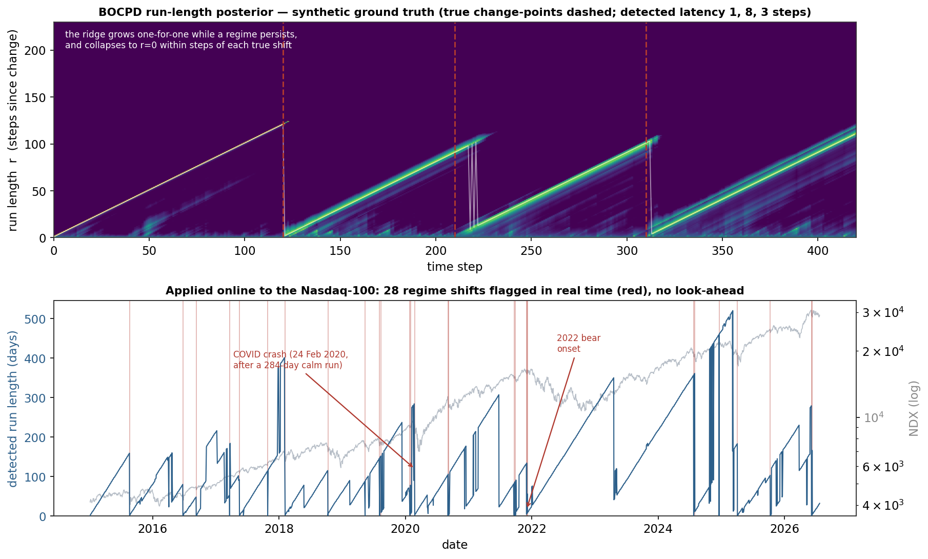
The mechanism is visible in the figure’s top panel — the signature BOCPD picture. While a regime persists, essentially all posterior mass sits on the run length that grows one-for-one with time: the bright diagonal ridge. When a change-point arrives, today’s observation is wildly unlikely under the old segment (\pi(x_t) collapses for large r), the reset branch dominates, and the mass jumps to r = 0 — the ridge falls off a cliff and a new one begins climbing from the floor. Detection is exactly this: watch the maximum-a-posteriori run length and flag a change when it collapses.
One honest implementation point, because it is where a naïve version fails and it is the kind of detail that separates a working detector from a copied formula. The intuitive alarm — threshold the change-point probability P(r_t = 0) — does not work on a long, noisy series: over thousands of returns that probability stays diffuse (its maximum here is about 0.004), because the mass spreads thinly across many candidate run lengths and no single step ever carries a clean spike. My first Nasdaq run, thresholding P(r_t=0), detected zero change-points and missed the COVID crash entirely. The robust online signal is the collapse of the MAP run length itself — a structural reset, not a probability peak — and switching to it turned the same model into the detector below. The failure was a lesson, not a dead end: the right observable was already in the posterior; I was reading the wrong one.
4. What did the demonstration show?
Ground truth first, as everywhere in this tier. I built a synthetic series with three known change-points (a volatility jump, a volatility drop with a mean shift, and a mean collapse) and ran BOCPD blind. It detected all three, at latencies of 1, 8, and 3 steps (top panel). The pattern is itself informative: the volatility explosion was caught in a single step — a sudden burst of large returns is the easiest break to see — while the volatility contraction took eight, because confirming that a regime has gone quiet requires accumulating several unremarkable observations. A detector you can trust is one you have first watched find answers you already knew.
Then the market. Run online over 2,903 daily Nasdaq-100 returns (Jan 2015 → Jul 2026), hazard 1/250, the detector flagged 28 regime shifts in real time, with no look-ahead (bottom panel). The headline result is the COVID crash, detected on 24 February 2020 — after the model had accumulated a 284-day calm run stretching back to mid-2019 — within days of the market top and using no future data whatsoever. The 2022 bear market was flagged on 1 December 2021, weeks before the index peaked; the February 2018 “volmageddon” and the Q4 2018 selloff appear too. The sawtooth in the figure is the whole story: the run length climbs steadily through each calm stretch and is cut down the instant turbulence arrives.
5. What are its strengths?
- Genuinely online. It uses only data up to now and updates in closed form each step — the property the HMM lacks and a live Regime Agent requires.
- Probabilistic, not a heuristic. The output is a full posterior over run length, so “how sure are we a regime changed?” has a real answer, not a tripped threshold.
- Fast latency on the shifts that matter. Volatility explosions — the breaks that destroy accounts — are caught fastest, as the synthetic and the COVID detection both show.
- Heavy-tailed by construction. The Student-t predictive tolerates the fat tails of returns instead of crying wolf at every three-sigma day.
- Interpretable and tunable. One knob, the hazard rate, sets the prior regime length; everything else is exact Bayesian updating.
6. What are its weaknesses?
- The i.i.d.-within-segment assumption is false for returns. Volatility clusters, so a “segment” is never truly stationary; BOCPD detects the big breaks robustly but will over-segment persistent turbulence.
- Detection latency is irreducible at the start of a shift. There is little evidence a regime has changed in its first day; a gentle drift (unlike a crash) can take many steps to confirm — the eight-step case.
- Read the right signal. As shown, thresholding P(r_t=0) fails on long series; you must monitor the run-length mode — a real trap for a careless implementation.
- Constant hazard is a simplification. A single expected regime length across a decade is crude; real markets switch at wildly varying frequencies.
- Abrupt-change model. BOCPD assumes breaks are sudden; slow structural drift is better handled by an explicitly time-varying model.
7. How could it apply to markets?
This is the proposal’s Regime Agent given a real-time sense. The HMM supplies the vocabulary of regimes (calm, turbulent, and their statistics) by learning from history; BOCPD supplies the live alarm that one regime has just handed off to another, point-in-time, with a probability attached. Together they let the downstream RL trading agent and the risk agent react to a developing shift — cut exposure, widen stops, switch the policy’s regime conditioning — before the loss is realised rather than after. The COVID detection is the proof of concept: a 284-day-calm system that raised its hand on 24 February 2020, days into the break, on past data alone. The caveats shape the design honestly: because the detector over-segments clustered volatility and lags gentle drifts, a deployed Regime Agent fuses BOCPD’s online alarm with the HMM’s structural labels and a GARCH volatility estimate rather than trusting any one — and, as always in this tier, the machinery was validated against known change-points before it was pointed at the market.
8. What does the Python code look like?
import numpy as np
from scipy.stats import t as student_t

def bocpd(x, hazard, mu0=0.0, kappa0=0.1, alpha0=1.0, beta0=1.0):
    """Online change-point detection. Returns the MAP run length at each step;
    a change-point is where it COLLAPSES (not where P(r=0) peaks)."""
    mu, kap, al, be = (np.array([v]) for v in (mu0, kappa0, alpha0, beta0))
    R = np.array([1.0])                                   # run-length posterior P(r_t | x_{1:t})
    MAP = np.zeros(len(x), int)
    for t, xt in enumerate(x):
        scale = np.sqrt(be * (kap + 1) / (al * kap))      # Student-t predictive from the NIG prior
        pred  = student_t.pdf(xt, df=2 * al, loc=mu, scale=scale)
        grow  = R * pred * (1 - hazard)                   # r -> r+1  (regime persists)
        reset = np.sum(R * pred * hazard)                 # r -> 0    (a change occurs)
        R = np.concatenate([[reset], grow]); R /= R.sum()
        MAP[t] = int(np.argmax(R))                        # the online detection signal
        # conjugate Normal-Inverse-Gamma update (new-segment prior prepended at r=0);
        # beta uses the OLD mu/kappa, so update it before overwriting them:
        be  = np.concatenate([[beta0],  be + kap * (xt - mu) ** 2 / (2 * (kap + 1))])
        mu  = np.concatenate([[mu0],    (kap * mu + xt) / (kap + 1)])
        kap = np.concatenate([[kappa0], kap + 1])
        al  = np.concatenate([[alpha0], al + 0.5])
    return MAP

# a change-point is flagged where the run length collapses:
MAP = bocpd((r - r.mean()).values, hazard=1/250)
changes = [t for t in range(1, len(MAP)) if MAP[t] < 12 and MAP[t-1] - MAP[t] > 25]
The loop is the whole algorithm: one Student-t predictive, a two-branch reweighting (grow vs reset), a conjugate parameter update, repeated once per observation. Detection reads the run-length mode’s collapse — the single most important line to get right.
9. How would I explain it to a supervisor?
“My HMM labels regimes, but it’s a smoother — it uses the whole history, so its labels contain look-ahead and can’t drive a live system. Bayesian online change-point detection fixes that. It tracks a posterior over the run length — time since the last regime change — and updates it exactly on each new return, with a Student-t predictive from a conjugate prior so it respects fat tails. While a regime holds, the most probable run length grows one-for-one with time; when the distribution breaks, that run-length estimate collapses to zero, and that collapse is the alarm. I validated it on synthetic data with known change-points — it caught all three, a volatility jump in a single step. Then I ran it online on eleven years of Nasdaq returns and it flagged twenty-eight regime shifts point-in-time, including the COVID crash on the 24th of February 2020 after a 284-day calm run, and the 2022 bear market weeks before the peak — no future data. One real lesson: the obvious signal, thresholding the change-point probability, fails on a long series because that probability stays diffuse; you have to watch the run-length mode collapse instead — which is what turned a detector that found nothing into one that found the crash. This is my Regime Agent’s real-time layer: the HMM gives the regime vocabulary, BOCPD gives the live alarm, and a risk layer acts on it before the drawdown, not after.”
Method: BOCPD (Adams–MacKay 2007) with a Normal-Inverse-Gamma prior (\mu_0=0,\ \kappa_0=0.1,\ \alpha_0=1,\ \beta_0=1) giving a Student-t predictive with 2\alpha dof; constant hazard H=1/250 (Nasdaq) and 1/100 (synthetic); exact untruncated run-length recursion. Detection = MAP run-length collapse (drop >25 to a floor <12), which the diffuse P(r_t=0) — max \approx 0.004 — does not provide. Data: NDX daily returns 2015-01-05 → 2026-07-22, n=2{,}903, de-meaned. Synthetic: four i.i.d. Gaussian segments, true change-points at 120/210/310, detected latencies 1/8/3 steps. Results: 28 online regime shifts; COVID crash detected 2020-02-24 (after a 284-day run), 2022 onset 2021-12-01. Every number was checked.