Markov Decision Processes & Bellman Equations

The formal language of sequential decisions — solved exactly on a real market regime model

An MDP formalises decision-making over time: states, actions, transitions, rewards, and a discount factor, tied together by the Bellman equation. Value iteration solves a regime-based position-sizing MDP built from this site’s fitted HMM — exactly, with a policy that quantifies what foresight is worth.

This entry opens a new tier of the library — the decision systems and reinforcement learning foundations of my PhD proposal — and it marks a genuine shift in question. Every supervised model so far asked what will happen next? An MDP asks the question a trader actually faces: what should I do now, given that today’s action shapes tomorrow’s position, costs, and options? The Markov Decision Process is the formal language for that problem, the Bellman equation is its central identity, and everything in reinforcement learning — from Q-learning to PPO — is a method for solving it when the model is unknown. Here the model is known, built from this site’s own fitted regime dynamics, so the MDP can be solved exactly — and the solution puts a number on something intuition can’t: what foresight is worth.

1. What problem does it solve?

Sequential decision-making under uncertainty: choosing actions over time, where each action brings immediate reward and changes the situation future decisions face. Prediction models optimise one-step accuracy; an MDP optimises a policy — a rule mapping every state to an action — against cumulative long-run reward. That distinction is exactly what the quant-specific section flagged as missing from supervised learning: no supervised model learns which sequences of decisions improve long-term risk-adjusted outcomes. The MDP is the framework in which that question is even well-posed.

2. What is the formalism?

An MDP is the tuple \mathcal{M} = (S, A, P, R, \gamma): a state space S, an action space A, transition probabilities P(s' \mid s, a), a reward function R(s,a), and a discount factor \gamma \in [0,1) weighting future against present reward. The Markov property does the heavy lifting: the state summarises everything the future needs from the past, so a policy need only depend on the current state. The objective is the expected discounted return G_t = \sum_{k=0}^{\infty} \gamma^k R_{t+k+1}, and the solution concepts are the value functions — V^\pi(s), the expected return from s under policy \pi, and the optimal V^*(s) and Q^*(s,a).

3. What is the Bellman equation?

The recursive identity that makes the infinite-horizon problem tractable. The optimal value of a state is the best immediate reward plus the discounted expected value of wherever you land:

V^*(s) \;=\; \max_{a \in A}\Big[\, R(s,a) \;+\; \gamma \sum_{s'} P(s' \mid s,a)\, V^*(s') \,\Big].

Its power comes from a fixed-point property: the Bellman operator is a \gamma-contraction, so it has a unique fixed point (V^*) and repeated application converges to it geometrically from any starting guess. That is value iteration — initialise V_0 = 0, apply the Bellman update until it stops changing — and the contraction guarantees the error shrinks like \gamma^k. (Its sibling, policy iteration, alternates policy evaluation with greedy improvement and typically converges in fewer, more expensive steps.) The greedy policy with respect to V^* is optimal — solving for values solves for behaviour.

4. How does it work on a real market model?

The demonstration builds an MDP from numbers this library has already fitted and verified. The regime entry’s hidden Markov model estimated two persistent market states — calm (\mu = +0.146%/day, \sigma = 0.76%) and turbulent (\mu = -0.072%/day, \sigma = 2.10%) — with transition matrix stay-probabilities 0.982 and 0.972. Those become the MDP’s dynamics. The state is (regime, current exposure); the action is choosing a new exposure w' \in \{0, 0.5, 1\}; the reward is risk-adjusted return minus a switching cost, r = w'\mu_s - \lambda (w'\sigma_s)^2 - c\,|w' - w|; and \gamma = 0.99.

Value iteration solves it exactly: 2,456 iterations to a final Bellman residual of 10^{-12}, with the error decaying geometrically at the contraction rate (the inset tracks \gamma^k). At a realistic 10bp switching cost the optimal policy is what economics predicts — fully invested in calm, flat in turbulence — with the state values quantifying the regimes: V^* \approx 5.7 starting calm versus 4.1 starting turbulent.

Left: the market MDP — the two HMM regimes as states (with their fitted means, volatilities and transition probabilities), exposure choices as actions, and a risk-adjusted reward with switching costs; solved exactly by value iteration. Right: the optimal action from (turbulent, fully long) as the switching cost rises. A myopic agent (γ≈0) stops de-risking fully at c ≈ 0.3% and entirely at c ≈ 0.7%; the far-sighted agent keeps paying to exit up to c₁ = 8.8% (fully) and c₂ = 33.8% (partially) because turbulence persists ~36 days. Inset: value iteration’s error decays as γᵏ — the Bellman contraction, visible.

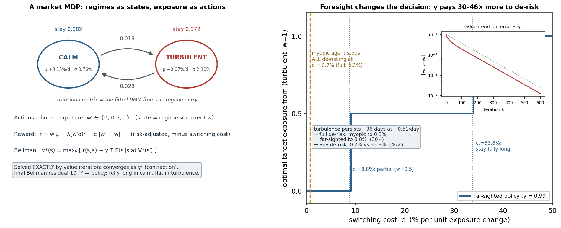
The right panel is the result that makes the formalism matter. Ask: starting turbulent and fully long, how much switching cost is it worth paying to de-risk? A myopic agent (\gamma \to 0) compares the cost only to today’s saving and stops de-risking fully once c exceeds 0.29%, and entirely above 0.73%. The far-sighted agent knows turbulence persists — the fitted expected duration is ~36 days — so avoiding it is worth roughly 36 \times 0.51 \approx 18 units, and value iteration shows it keeps paying to exit fully up to c_1 = 8.8% and partially up to c_2 = 33.8% (exploiting the quadratic risk penalty: halving exposure removes three-quarters of the variance). Foresight changes the willingness to pay by 30–46×, and the discount factor is precisely the dial that encodes it. At c = 2%, the two agents make opposite decisions from identical information: the myopic one stays fully long, the far-sighted one goes flat.

5. What are its strengths?

• The right objective. It optimises cumulative risk-adjusted outcomes over time — the thing a trading operation actually cares about — not one-step prediction accuracy.
• Exactly solvable when the model is known. Value/policy iteration deliver the provably optimal policy, with convergence guaranteed by the contraction.
• Makes trade-offs explicit and quantitative. Switching costs versus regime persistence, present versus future — the policy thresholds are numbers, not intuitions.
• The foundation of everything ahead. Q-learning, policy gradients and PPO are all methods for solving an MDP whose P and R are unknown; the formalism is the common language.
• Composable with this library. The regime HMM plugs in as the transition model; risk measures plug in as the reward — the pieces already exist.

6. What are its weaknesses?

• The Markov assumption is a modelling choice. If the chosen state omits relevant history, the “optimal” policy is optimal for the wrong problem — state design is where the craft lives.
• The true market model is unknown. Real P and R must be estimated (as here, from an HMM) or learned from interaction — which is exactly what reinforcement learning exists for.
• Curse of dimensionality. Exact solution enumerates states; realistic state spaces explode, forcing function approximation (the deep-RL entries ahead).
• Garbage in, optimal garbage out. The policy is exactly as good as the model: mis-estimated regime persistence would shift every threshold in the figure.
• The market is only partially observable. The true regime is latent — which the next refinement addresses directly.

7. How could it apply to markets?

This entry is the application — and it is the load-bearing formalism of the PhD proposal. The proposal’s RL Trading Agent lives inside exactly this structure: states combining regime probabilities, news features and holdings; actions over exposure; a risk-sensitive reward penalising variance, drawdown, costs and turnover. And the bridge from this entry to the proposal is elegant: because the true regime is hidden, the honest formulation is a partially observable MDP, where the agent acts on a belief b_t(s) = P(S_t = s \mid o_{1:t}) over latent states — and that belief is precisely the HMM forward filter this library already built. The filtered regime probability isn’t just a risk dial; it is the belief state of a POMDP, which turns the regime-scaled exposure rule from that entry into a first, hand-crafted policy — one that reinforcement learning, in the entries ahead, will try to learn and improve. The practical takeaway carries the site’s honest thread forward: the MDP machinery optimises how to act on structure that exists (regimes, persistence, costs) — it does not conjure predictability, it allocates against it.

8. What does the Python code look like?

import numpy as np

# states: (regime, current exposure); actions: choose new exposure
def value_iteration(states, actions, P, R, gamma=0.99, tol=1e-12):
    V = {s: 0.0 for s in states}
    while True:
        V_new, policy = {}, {}
        for s in states:
            q = {a: R(s, a) + gamma * sum(P(s2, s, a) * V[s2] for s2 in states)
                 for a in actions}                       # the Bellman update
            policy[s] = max(q, key=q.get)
            V_new[s]  = q[policy[s]]
        if max(abs(V_new[s] - V[s]) for s in states) < tol:
            return V_new, policy                         # V*, and the greedy-optimal policy
        V = V_new
# contraction guarantee: the error shrinks like gamma**k — convergence is not a hope, it's a theorem

The whole algorithm is the Bellman equation applied until it stops changing. gamma is the foresight dial: at 0 the agent is myopic; at 0.99 it plans ~100 days ahead — and as the figure shows, that single parameter can reverse the optimal decision.

9. How would I explain it to a supervisor?

“An MDP formalises sequential decision-making: states, actions, transition probabilities, rewards, and a discount factor, with the Markov property letting a policy depend only on the current state. The Bellman equation defines the optimal value recursively — best immediate reward plus discounted expected value of the successor — and because the Bellman operator is a γ-contraction, value iteration converges geometrically to the unique optimum. I built one from my own fitted regime model: HMM states as dynamics, exposure as the action, risk-adjusted return minus switching costs as the reward, solved exactly to a 10⁻¹² residual. The policy is fully invested in calm and flat in turbulence, and the interesting result is what foresight is worth: a myopic agent stops paying to fully de-risk at a third of a percent of switching cost, while the γ = 0.99 agent keeps paying up to nine percent, because turbulence persists for a month — a thirty-fold difference from the discount factor alone. Since the true regime is latent, the honest extension is a POMDP whose belief state is exactly my HMM’s forward filter — which is the formal foundation of my proposed RL trading agent, and what Q-learning and PPO, next, will learn without knowing the model.”

MDP constructed from the regime entry’s fitted HMM (state means/volatilities and transition matrix, daily Nasdaq-100 data); risk aversion \lambda = 0.1, \gamma = 0.99, exposure grid \{0, 0.5, 1\}. Solved by value iteration to a Bellman residual of 9.8 \times 10^{-13} in 2,456 iterations; contraction rate, policy thresholds (c_1 = 8.8%, c_2 = 33.8%; myopic thresholds 0.29% and 0.73%, confirmed analytically) found by bisection on the exact solution. This entry begins the decision-systems & RL tier of the PhD roadmap. Every number was checked.