Ensemble Methods & Model Combination
Equal weighting, majority vote, Bayesian model averaging and stacking — and the diversity that decides whether combining helps at all
Every model in this library outputs a probability, and the proposal’s architecture ends in a layer that must combine the probabilities of many specialist models into one market-state estimate. Before any clever hypothesis-reconciliation mechanism can earn its place, it has to beat the boring, battle-tested ways of combining models: equal weighting, majority vote, Bayesian model averaging and stacking. These are the consensus baselines named in the proposal, and this entry builds all four, tests them honestly, and extracts the one law that governs whether combining models helps at all — diversity, not count. The result is deliberately humbling, and it is exactly the kind of finding that should shape an architecture rather than flatter it.
1. What problem does it solve?
Turning many models into one better, better-calibrated model — sometimes. No single model is right in every regime: a linear model is stable but blind to interactions, a boosted tree is sharp but over-confident, a volatility-persistence rule is robust but crude. Combining them can reduce variance, smooth over individual failure modes, and improve calibration. But “can” is load-bearing. The central question this entry answers is not how to combine models — that part is easy — but when combining is worth anything, and the honest answer turns on how correlated the models’ errors are. For the proposal, these four combiners are the yardstick (RQ5): a bounded consensus layer that reconciles competing hypotheses only justifies its complexity if it beats plain averaging.
2. The four combiners
Given M base models producing probabilities p_{i,t} for a binary event, the standard combiners are:
- Equal weighting — the average \bar p_t = \frac{1}{M}\sum_i p_{i,t}. No parameters, nothing to over-fit; the “1/N” rule that is famously hard to beat.
- Majority vote — each model casts a hard 0/1 vote at a threshold and the ensemble reports the fraction voting yes. Simple, but it throws away the probabilities, keeping only their sign.
- Bayesian model averaging (BMA) — weight each model by its posterior credibility, w_i \propto \exp\!\big(\sum_{t\in\text{val}} \log p_i(y_t)\big), i.e. its cumulative predictive log-score on held-out data, then average \sum_i w_i\, p_{i,t}. Good predictors get more weight.
- Stacking — fit a meta-model (here a logistic regression) whose inputs are the base models’ predictions, trained on held-out base predictions to learn the best blend. The most flexible, and the most prone to over-fit.
The discipline that makes this honest is the split: base models are trained on a train window, BMA weights and the stacking meta-model are fit on a separate validation window, and every number below is measured on a test window none of them ever saw.
3. An honest market test — on a target that is actually predictable
Combining models is pointless on a target with no signal, so I deliberately avoided next-day direction (which this site shows again and again is a coin toss, AUC ≈ 0.50) and chose one that is genuinely forecastable: next-day turbulence — whether tomorrow’s absolute Nasdaq return exceeds the train-set 70th percentile (a 1.0% move). Because volatility clusters, this is predictable, and the four base models confirm it, all scoring AUC ≈ 0.67 — far above chance. That contrast is the whole thesis of the site in one line: direction is noise, turbulence is structure.
Four base models read that structure: a logistic regression on volatility features (AUC 0.669), a gradient-boosted tree (0.671), a random forest (0.670), and a pure EWMA volatility-persistence model (0.601, the weak-but-different one). Then the four combiners:
| Method | AUC | Brier | ECE |
|---|---|---|---|
| Best single base (random forest) | 0.670 | 0.2102 | 0.052 |
| Equal weighting | 0.670 | 0.2111 | 0.046 |
| Bayesian model averaging | 0.672 | 0.2099 | 0.046 |
| Stacking | 0.672 | 0.2157 | 0.072 |
| Majority vote | 0.593 | 0.2928 | 0.266 |
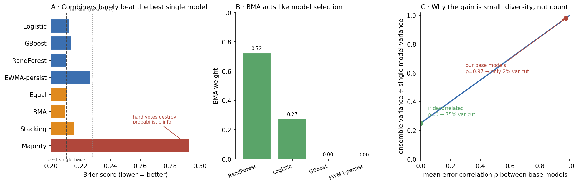
The story is not “the ensemble wins big.” It is far more instructive. BMA is the best method — but it beats the best single model by a hair (0.2099 vs 0.2102), and it does so by essentially turning into model selection: its weights collapse onto the random forest (0.72) and logistic (0.27), zeroing the other two. Equal weighting ties the best base and improves its calibration (ECE 0.052 → 0.046). Stacking over-fits the modest validation set and comes out worse than plain averaging. Majority vote is a disaster — by discarding the probabilities and keeping only hard votes it destroys the very information a probabilistic system needs, wrecking both Brier (0.29) and log-loss (8.6). The fancy combiner did not dominate the simple one, and the simplest hard combiner failed outright.
4. Why the gain was tiny — the one law that matters
The reason combining barely helped is not the choice of combiner; it is that the base models were 0.97-correlated in their errors. The variance-reduction identity makes this exact. For an equal-weight average of M models with equal error variance \sigma^2 and average pairwise error-correlation \rho,
\frac{\operatorname{Var}(\bar p)}{\sigma^2} \;=\; \frac{1 + (M-1)\rho}{M}.
With M=4 and \rho = 0.974 this is 0.98 — a 2% variance reduction, exactly the microscopic Brier improvement observed. Had the four models been decorrelated (\rho = 0), the same four would cut variance to 0.25 — a 75% reduction. An ensemble’s benefit comes from diversity, not from the number of models. Four models that all read the same volatility signal are almost one model wearing four hats; their consensus is barely better than any one of them.
5. What are its strengths?
- Variance reduction for free — when models are diverse. Averaging decorrelated, comparably-accurate models is the closest thing to a free lunch in forecasting; the identity above quantifies exactly how much.
- Equal weighting is a ferociously strong baseline. With no parameters it cannot over-fit, and it here matched the best single model and improved its calibration — the “1/N” lesson that humbles more elaborate schemes.
- BMA degrades gracefully. When one model dominates, BMA concentrates on it (behaving like selection); when several are comparable, it spreads weight — a principled, self-adjusting compromise.
- Model-agnostic and cheap. All four sit on top of any set of probabilistic models, so every specialist in the architecture can feed a consensus layer without being rebuilt.
- Calibration often improves. Even a marginal accuracy gain from averaging tends to pull probabilities toward honesty (ECE 0.052 → 0.046 here), which is what a risk-sizing system actually consumes.
6. What are its weaknesses?
- Correlated bases give almost nothing. The headline failure mode, shown directly: ρ = 0.97 → a 2% variance cut. Stacking more copies of the same view is wasted effort.
- Stacking over-fits. A meta-model has parameters, and on a modest validation window it learned noise and lost to plain averaging — the classic bias–variance trap of the most flexible combiner.
- Hard voting destroys information. Majority vote discards probabilities; for any downstream system that multiplies by confidence, it is strictly worse than averaging the probabilities themselves.
- Weights assume the future looks like validation. BMA and stacking weights are fit on one period; a regime shift can make yesterday’s best model today’s worst, so static weights are fragile — the motivation for adaptive weighting (the next entry) and for conditioning weights on regime.
- Garbage in, garbage out. Averaging cannot manufacture skill that no base model has; on a no-signal target (direction), every combiner would sit at the no-skill line.
7. How could it apply to markets?
This is the proposal’s consensus layer in baseline form, and the demonstration draws its blueprint. First, it sets the bar for RQ5: the bounded hypothesis-reconciliation mechanism must beat these combiners, not a strawman — and beating a well-built BMA or equal-weight is a genuinely high bar. Second, and more consequentially, it explains a core architectural choice. The reason to assign specialists to different evidence domains — trend, volatility, liquidity, macro narrative, cross-asset — rather than stacking many models on the same features, is precisely to manufacture the decorrelation that the variance identity says an ensemble needs. Diversity is not a nicety of the design; it is the entire source of the consensus layer’s value. Third, it previews H7: adaptive expert weighting should beat equal weighting, but not necessarily by much, because transparent baselines are strong — here BMA’s edge over 1/N was two Brier ten-thousandths. A proposal that already knows its fancy layer must fight for every basis point against a parameter-free baseline is one built on evidence. The next step is the adaptive version — weights that update online and condition on the current regime — which is where combining models can finally earn more than a rounding error.
8. What does the Python code look like?
import numpy as np
from sklearn.linear_model import LogisticRegression

# base-model probabilities on validation and test: columns = models
# Pva (n_val x M), Pte (n_test x M); yva = validation labels

# --- Equal weighting: the parameter-free baseline that is hard to beat ---
equal = Pte.mean(axis=1)

# --- Bayesian model averaging: weight by validation predictive log-score ---
eps = 1e-6; Pc = np.clip(Pva, eps, 1 - eps)
loglik = (yva[:, None] * np.log(Pc) + (1 - yva[:, None]) * np.log(1 - Pc)).sum(axis=0)
w = np.exp(loglik - loglik.max()); w /= w.sum()          # collapses onto the best models
bma = Pte @ w

# --- Stacking: a logistic meta-model on the base predictions (fit on validation only) ---
stack = LogisticRegression(max_iter=2000).fit(Pva, yva).predict_proba(Pte)[:, 1]

# --- The law that decides if any of this helps: diversity, not count ---
err = Pte - yte[:, None]                                  # signed errors per model
rho = np.corrcoef(err.T)[np.triu_indices(Pte.shape[1], 1)].mean()
var_ratio = (1 + (Pte.shape[1] - 1) * rho) / Pte.shape[1] # ~1 when correlated, ~1/M when not
The combiners are three lines each; the fourth block is the one that matters, because it tells you whether the first three were worth running.
9. How would I explain it to a supervisor?
“Combining models is the last layer of my architecture, so I built the four standard combiners — equal weighting, majority vote, Bayesian model averaging and stacking — and tested them honestly on a target that actually has signal: next-day turbulence, which is forecastable at AUC 0.67, unlike direction. The result was instructive rather than flattering. BMA was the best method but beat the best single model by one Brier ten-thousandth, and it did so by concentrating its weight on the two best models — it behaved like model selection. Equal weighting tied the best base and improved its calibration. Stacking over-fit the validation set and did worse. Majority vote was catastrophic because it throws the probabilities away. The reason the gains were tiny is the whole point: my four base models were 0.97-correlated, and the variance-reduction identity says an equal-weight ensemble only cuts error variance to (1+(M−1)ρ)/M — 98% of the original at that correlation, versus 25% if they were decorrelated. So an ensemble’s value comes from diversity, not count. That is exactly why my proposal assigns specialists to different evidence domains instead of stacking models on the same features — the architecture manufactures the decorrelation that makes a consensus layer worth having. And it sets an honest, high bar for my hypothesis-reconciliation layer: it has to beat a well-built BMA, not a strawman.”
Data: NDX daily 2015–2026 (2,866 usable rows after warm-up). Target: next-day turbulence, |r_{t+1}| above the train 70th percentile (|r| = 1.01\%); test base-rate 0.350. Chronological split train 1,719 / validation 573 / test 574; turbulence threshold, feature scaling and base models fit on train, BMA weights and stacking meta-model fit on validation, all metrics on test. Base models (test AUC / Brier / ECE): logistic 0.669 / 0.2122 / 0.054; gradient boosting 0.671 / 0.2136 / 0.062; random forest 0.670 / 0.2102 / 0.052; EWMA-persistence 0.601 / 0.2263 / 0.073. Combiners: equal 0.670 / 0.2111 / 0.046; BMA 0.672 / 0.2099 / 0.046; stacking 0.672 / 0.2157 / 0.072; majority-vote 0.593 / 0.2928 / 0.266 (log-loss 8.64). BMA weights: random forest 0.725, logistic 0.274, gradient boosting 0.001, EWMA 0.000. Mean pairwise error-correlation ρ = 0.974; equal-weight variance-reduction factor (1+(M-1)\rho)/M = 0.98 at that ρ vs 0.25 at ρ = 0. ECE with 15 equal-width bins. Every number was checked.