The Kalman Filter & State-Space Models
Optimal real-time estimation of a hidden, drifting state — the linear-Gaussian filter behind trend extraction, time-varying beta, and the belief state a POMDP needs
The regime and Markov-switching entries estimated a discrete hidden state. This one estimates a continuous hidden state that drifts through time — a level, a slope, a beta — from noisy observations, optimally and in real time, and it does so with an honest measure of its own uncertainty. The Kalman filter is the linear-Gaussian workhorse of state estimation, and it sits at two points in the proposal: it is a Trend & persistence specialist (a real-time estimate of the market’s current level and drift), and it is the belief filter — the b_t a partially observable decision process requires. It is also the exact linear-Gaussian analogue of the HMM forward filter, so it inherits the site’s most important distinction: filtered (what you know now) versus smoothed (what you would know with hindsight).
1. What problem does it solve?
Tracking a hidden thing that moves, before you have all the data. Many quantities a market system cares about are latent and non-stationary: the “true” price level under microstructure noise, the current drift of a trend, a stock’s exposure to the market. You never observe them directly, they change over time, and you must estimate them now — not with the luxury of the whole sample. The Kalman filter is the provably optimal (minimum-mean-square-error) recursive estimator for this problem under linear-Gaussian assumptions, and — crucially for a system that sizes risk — it reports not just an estimate but a covariance, an honest statement of how uncertain it is. It replaces the two clumsy alternatives — a fixed look-back window (arbitrary length, equal weights, laggy) and a static regression (assumes nothing drifts) — with a principled, self-tuning, real-time estimate.
2. The state-space model and the recursion
A linear-Gaussian state-space model has a hidden state x_t that evolves, and a noisy observation y_t of it:
x_t = F x_{t-1} + w_t,\quad w_t\sim N(0,Q); \qquad y_t = H_t x_t + v_t,\quad v_t\sim N(0,R).
The Kalman filter carries the state estimate and its covariance forward in two steps. Predict — push the state through the dynamics and let uncertainty grow: \hat x_{t|t-1}=F\hat x_{t-1}, P_{t|t-1}=FP_{t-1}F^\top+Q. Update — correct by the innovation \tilde v_t = y_t - H_t\hat x_{t|t-1}, weighting it by the Kalman gain K_t = P_{t|t-1}H_t^\top S_t^{-1} with S_t=H_tP_{t|t-1}H_t^\top+R: \hat x_{t}=\hat x_{t|t-1}+K_t\tilde v_t. The gain is the whole story — it is the optimal blend of what the model predicted and what was observed, and it self-adjusts: high when the state is uncertain or the sensor is clean, low when the observation is noisy. The result is a belief b_t = N(\hat x_{t},P_{t}), a full posterior over the hidden state. A backward pass (the RTS smoother) then computes the smoothed estimate that conditions on the entire sample — cleaner, but no longer real-time. (Two asides that tie the site together: the steady-state gain of the simplest model is exactly an EWMA, and this whole recursion is the Gaussian version of the HMM forward filter.)
3. Verifying the machinery, then trusting it
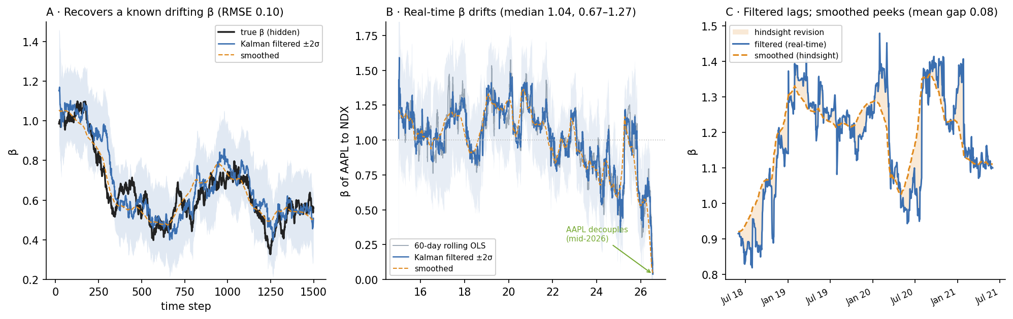
No estimator goes on this site until it is checked against something known. Two checks. First, against a reference implementation: my from-scratch filter run as a local-level model on the Nasdaq log-price reproduces statsmodels’ filtered state to a maximum absolute difference of 2.8 × 10⁻¹⁰ — the same recursion, to ten decimals. Second, against ground truth: I simulated a known randomly-drifting β and asked the filter to recover it. Maximum likelihood recovered the process-noise and observation-noise variances almost exactly (estimated q_\beta = 1.72\times10^{-4} vs true 1.67\times10^{-4}; R =
6.5\times10^{-5} vs 6.4\times10^{-5}), the filtered β tracked the hidden truth with RMSE 0.095, the smoothed β did better at 0.068, and — the honesty check that matters most — the true β fell inside the filter’s own ±2σ band 95.9% of the time. The filter’s stated uncertainty is real, not decorative.
4. An honest market demonstration — time-varying beta
A stock’s β to the market is usually assumed constant; it is not. Modelling r^{\text{AAPL}}_t = \alpha_t + \beta_t\, r^{\text{NDX}}_t + v_t with \beta_t a random walk turns the Kalman filter into a real-time beta estimator. Over 2015–2026, AAPL’s filtered β to the Nasdaq drifts substantially — median 1.04, with a 10–90% range of 0.67 to 1.27 — and the filter tracks it with an uncertainty band instead of a guess. It agrees closely with a 60-day rolling OLS beta (correlation 0.94) but is the better object: no arbitrary window length (the process-noise variance is estimated by MLE), a proper uncertainty band, and a faster, principled response — it even caught AAPL’s brief decoupling from the Nasdaq in mid-2026, when β fell toward zero as the index sold off and the stock held. Set against the Markov-switching beta, which jumps discretely between regimes, the Kalman beta drifts continuously — two honest models of the same non-stationarity, and the proposal can use either as the situation demands.
5. The filtered-vs-smoothed lesson, in linear-Gaussian form
The right panel is the point the whole site keeps making. The smoothed β is cleaner and turns earlier — but only because it conditions on the future. It revises the real-time filtered estimate by a mean of 0.076 in β units, and those revisions use data that did not exist yet. A backtest that sizes a hedge on the smoothed β would look wonderful and be a fiction; a live desk has only the filtered β, which lags the turns. This is the identical trap flagged in the Hamilton filter and regime entries, now in continuous form, and it is why the proposal insists every specialist emit its filtered estimate. The smoother is for research and attribution, never for a decision made at time t.
6. What are its strengths?
- Optimal, recursive, real-time. Under linear-Gaussian assumptions it is the minimum-variance estimator, computed online in closed form — no window, no refit, one cheap update per observation.
- It quantifies its own uncertainty. The covariance P_t is a first-class output, verified here to cover the truth 95.9% of the time — exactly what a risk-sizing system needs.
- No arbitrary window. The process-noise variance Q is estimated by maximum likelihood, replacing the rolling-window length with a data-driven adaptivity dial.
- General and composable. The same recursion does trend extraction, time-varying regression, and sensor fusion, and it is the belief filter for a linear-Gaussian POMDP — the b_t the decision layer consumes.
- Filtered vs smoothed is explicit. The framework separates the real-time estimate from the hindsight one by construction, so look-ahead cannot sneak in unnoticed.
7. What are its weaknesses?
- Linear-Gaussian is an assumption, not a fact. Fat tails and nonlinearity break optimality; markets have both, so the filter is a useful approximation that the extended/unscented/particle filters exist to relax.
- Garbage variances, garbage state. Q and R (or their MLE) drive everything; too large a Q lets the state over-wander, too small makes it deaf to real change — the same bias–variance dial as a window length, only continuous.
- The filtered estimate lags the turn. Real-time is not free: at the moment a β actually shifts, the filter is still catching up — the unavoidable cost the smoother hides.
- A state estimate is not a signal. Letting β drift improved one-step return fit only marginally (RMSE 112.9 → 110.1 bps); the filter tells you the current exposure honestly, it does not predict returns.
- Model structure must be right. A random-walk state, the wrong F, or an omitted component all mis-estimate the thing you wanted — the model is only as good as its specification.
8. How could it apply to markets?
In the proposal the Kalman filter wears three hats. It is the Trend & persistence specialist: a real-time estimate of the market’s level and drift, emitted with its uncertainty so the consensus layer can weight it by confidence rather than treat it as a point. It is a real-time exposure and hedge-ratio estimator — the time-varying β here is precisely the number a risk overlay needs to neutralise market exposure as it drifts, and doing it with a filter rather than a rolling window removes an arbitrary choice and adds an honest error bar. And it is the belief filter that makes the partially-observable framing operational: the b_t = N(\hat x_t, P_t) it produces is the continuous-state cousin of the regime posterior, the object a decision or risk agent conditions on. The deepest connection is methodological: filtering is the act of turning a stream of noisy observations into a current best estimate of a hidden state with calibrated uncertainty — which is the entire job of the architecture’s lower layers. The Kalman filter is the cleanest, most rigorous instance of that job, and the discipline it enforces — estimate the state, state your uncertainty, and never let the smoother’s hindsight leak into a live decision — is the discipline the whole system is built on.
9. What does the Python code look like?
import numpy as np

def kalman(y, Hs, F, Q, R, x0, P0):
    """Filter a scalar series y with time-varying observation rows Hs[t] (1 x n)."""
    T, n = len(y), len(x0)
    xf, Pf = np.zeros((T, n)), np.zeros((T, n, n))
    xp, Pp = np.zeros((T, n)), np.zeros((T, n, n))       # predicted moments (for the smoother)
    x, P, llf = x0.copy(), P0.copy(), 0.0
    for t in range(T):
        x = F @ x;  P = F @ P @ F.T + Q                   # predict
        xp[t], Pp[t] = x, P
        H = Hs[t];  S = (H @ P @ H.T).item() + R          # innovation variance
        v = (y[t] - H @ x).item()                         # innovation
        K = (P @ H.T).ravel() / S                         # Kalman gain
        x = x + K * v;  P = P - np.outer(K, H @ P)        # update
        xf[t], Pf[t] = x, P
        llf += -0.5 * (np.log(2*np.pi*S) + v*v/S)         # log-likelihood (for MLE of Q, R)
    return xf, Pf, xp, Pp, llf

def rts_smoother(xf, Pf, xp, Pp, F):                      # backward pass -> smoothed (hindsight)
    xs, Ps = xf.copy(), Pf.copy()
    for t in range(len(xf) - 2, -1, -1):
        C = Pf[t] @ F.T @ np.linalg.inv(Pp[t+1])
        xs[t] = xf[t] + C @ (xs[t+1] - xp[t+1])
        Ps[t] = Pf[t] + C @ (Ps[t+1] - Pp[t+1]) @ C.T
    return xs, Ps
For time-varying β, the state is [\alpha_t,\beta_t], F=I, and each observation row is Hs[t] = [[1, r_market[t]]]; maximising llf over the noise variances is the whole calibration.
10. How would I explain it to a supervisor?
“The Kalman filter estimates a hidden state that drifts over time, optimally and in real time, and reports its own uncertainty. I implemented it from scratch and checked it two ways: it reproduces statsmodels’ filtered state to ten decimals, and on synthetic data with a known randomly-drifting β it recovered the noise parameters, tracked the truth, and its 2-sigma band covered the true value 96% of the time — so the uncertainty is honest. Then I used it for time-varying beta: AAPL’s β to the Nasdaq isn’t constant, it drifts from about 0.67 to 1.27 with a median near 1.04, and the filter tracks it in real time with an error band and no arbitrary window — it even caught AAPL briefly decoupling from the index in 2026. Two lessons for my proposal. First, this is the continuous-state version of my regime filter and the belief state a POMDP needs — estimate the hidden state, state your uncertainty. Second, it makes the filtered-versus-smoothed point exactly: the smoothed beta is cleaner and turns earlier, but only because it uses the future — it revises the real-time estimate by about 0.08 — so a live system must use the filtered value and a backtest must never use the smoothed one. And the honest limit: a real-time state estimate is not a return signal — letting beta drift barely improved return fit. It tells you your exposure truthfully; it doesn’t predict the market.”
Kalman filter and RTS smoother implemented from scratch. Machinery check: filtered state vs statsmodels UnobservedComponents('local level') on NDX log-price, max abs difference 2.8 × 10⁻¹⁰. Synthetic (T = 1500, random-walk β): MLE q_\beta = 1.72\times10^{-4} (true 1.67\times10^{-4}), R =
6.51\times10^{-5} (true 6.40\times10^{-5}); filtered β RMSE 0.095, smoothed 0.068; ±2σ coverage 0.959. Real: r^{\text{AAPL}}_t=\alpha_t+\beta_t r^{\text{NDX}}_t+v_t, [\alpha_t,\beta_t] random walk, daily 2015–2026 (2,903 obs), MLE noise variances, diffuse-ish init. Filtered β median 1.04, 10–90% range 0.67–1.27, brief mid-2026 decoupling toward ~0.04 (31 of 2,903 days below 0.4); mean ±2σ width 0.66; correlation with 60-day rolling OLS β 0.94; look-ahead mean |smoothed − filtered| = 0.076; one-step return-fit RMSE 112.9 bps (constant β) vs 110.1 bps (lagged filtered β, no look-ahead). Every number was checked.