Liquidity-Stress Anomaly Detection

Learning what ‘normal’ market conditions look like, and flagging the departures — the unsupervised tripwire of the liquidity specialist

The liquidity specialist’s detector: unsupervised anomaly detection on microstructure-stress features. An Isolation Forest recovers injected anomalies at 0.95 precision/recall, and on the Nasdaq it flags 5% of days that concentrate 5.4× into known crises and precede sharply higher volatility (41.6% vs 17.3% forward). Crucially, 18% of its flags are ‘quiet illiquidity’ — wide intraday ranges with no big close-to-close move — exactly the stress a simple return threshold misses.

The cross-asset and structural-change specialists watch relationships and breaks; the liquidity specialist watches conditions — is the market functioning normally, or is it stressed, thin and prone to gapping? That question has no natural label, so it is a job for unsupervised anomaly detection: learn what normal trading looks like from the data itself, and flag the days that do not belong. This entry builds that detector, verifies it recovers known anomalies, and shows on the Nasdaq that it catches real liquidity stress — including the kind a naive “big move” rule misses. It is the proposal’s liquidity-condition estimator, and the tripwire that tells the risk layer the market has become dangerous to trade. Its supervised counterpart turns the same features to a forward question — forecasting the coming week’s stress as a calibrated probability.

1. What problem does it solve?

Recognising abnormal, stressed market conditions without being told what they look like. Liquidity stress — widening spreads, collapsing depth, gapping prices, whipsaw ranges on thin volume — is rare, varied, and unlabelled, so you cannot train a classifier on it. What you can do is characterise normal conditions, which are abundant, and measure how far each day departs from them. Anomaly detection does exactly this: it fits the shape of the ordinary and scores the extraordinary. For a decision system this is the difference between “the price moved” and “the market broke” — and it is a condition signal, feeding the risk layer and the risk-on/off verdict, not a return forecast.

2. The features and the detectors

Real microstructure needs order-book data — spreads, depth, order imbalance — which this site does not have, so the honest version here builds a daily proxy of stress from OHLCV: the intraday range (H-L)/C, the absolute return |r|, the overnight gap, a volume z-score, and an Amihud illiquidity measure |r| / (\text{relative volume}) — price impact per unit of trading, high when a move happens on thin volume. Two complementary detectors learn “normal” from these. The Isolation Forest builds random trees that partition the feature space; anomalies, being sparse and far from the crowd, are isolated in very few splits, so a short average path length is the anomaly score — fast, non-parametric, and effective in several dimensions. The robust Mahalanobis distance, D^2=(x-\mu)^\top\Sigma^{-1}(x-\mu) with \mu and \Sigma from a minimum-covariance-determinant fit (so the outliers do not corrupt the estimate of normal), flags points beyond a \chi^2 threshold — interpretable, but assumes an elliptical cloud.

3. Verifying it recovers known anomalies

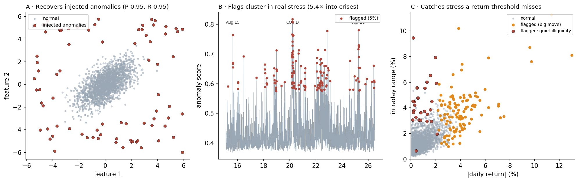
Since stress is unlabelled on real data, the check is on synthetic data where the truth is known: a correlated Gaussian cloud of “normal” points with a scatter of injected outliers (left panel). The Isolation Forest recovers them at 0.95 precision and 0.95 recall — it finds the anomalies and rarely cries wolf. The robust Mahalanobis detector catches all of them (recall 1.00) but at lower precision (0.45): it over-flags, because the uniform outliers do not form the ellipse its distance assumes. That contrast is itself the lesson — the Isolation Forest makes no shape assumption and is the sharper tool for messy, multi-dimensional stress features, so it drives the real-data analysis, with Mahalanobis as an interpretable cross-check.

Left: on synthetic data an Isolation Forest recovers injected anomalies (red) scattered around a correlated normal cloud (grey) at 0.95 precision and recall. Middle: on the Nasdaq the anomaly score over 2015–2026, with the 5% flagged days (red) clustering in real stress — the COVID crash, the August 2015 flash crash, 2022, and April 2025 — 5.4× more concentrated in crisis windows than chance. Right: intraday range versus absolute return — the detector flags the obvious big-move days (orange) but also ‘quiet illiquidity’ days (red) with wide ranges and small close-to-close returns, the stress a simple return threshold misses.

4. On the Nasdaq — and what a multivariate view adds

Run on the daily stress features with a 5% contamination rate, the Isolation Forest flags 144 of 2,867 days, and they are the right ones. Where crisis windows make up 10% of the sample, they contain 53% of the flagged days — a 5.4× concentration — and the top anomalies are precisely the episodes a trader would name: the March 2020 COVID cluster, the August 2015 flash crash, late 2022, and April 2025. More tellingly, the flags are economically meaningful: the five-day-forward realised volatility after a flagged day is 41.6%, against 17.3% on normal days — stress detected today genuinely precedes a more dangerous market, which is what makes the signal worth having.

The payoff of a multivariate detector over a simple “big return” rule is the sharpest result. Of the 144 flags, 26 (18%) are not even top-decile absolute-return days — they are days of wide intraday range (4.3% on average, versus 1.3% normal) with only a modest close-to-close move: whipsaw, gapping and intraday dislocation that a return threshold sails straight past but that are unmistakable liquidity stress. The right panel shows them — the red points hugging the left axis, low return but high range. A one-dimensional rule cannot see them; a detector watching the joint distribution of range, volume and impact can.

5. What are its strengths?

• Unsupervised — no labels needed. It learns “normal” from abundant ordinary data and flags departures, so it works precisely where stress is too rare and varied to label, and it can catch novel stress it has never seen.
• Multivariate — it sees what one feature can’t. The quiet-illiquidity result is the point: joint structure across range, volume and impact reveals stress that any single series (like the return) misses.
• Economically validated. Flags concentrate 5.4× in crises and precede 2.4× higher forward volatility — the score tracks something real, not just statistical outlyingness.
• Fast and robust. The Isolation Forest is non-parametric, scales to many features and observations, and needs no distributional assumption — an always-on condition monitor.
• A clean condition signal. It emits a stress probability the risk layer and the risk-on/off verdict can consume directly, distinct from any return view.

6. What are its weaknesses?

• “Normal” is defined by the training data, and it drifts. A detector fit on calm years over-flags in a persistently higher-volatility regime; the reference distribution must be maintained, the same non-stationarity problem as everywhere on this site.
• No ground truth. Being unsupervised, it cannot be scored directly — only validated indirectly (face validity, forward volatility), so its precision is never certain.
• Daily OHLCV is a proxy. Genuine liquidity lives in spreads, depth and order-flow; the range/volume/impact features approximate it and the real specialist would use an order-book feed.
• The contamination rate is a chosen knob. How much to flag is a false-alarm-versus-miss decision, exactly like CUSUM’s threshold — a risk choice, not a default.
• It flags stress, not cause or direction. An anomaly says “abnormal,” not “abnormal because of X” or “so prices will fall”; it is a condition monitor, and correlated features can dominate the score.

7. How could it apply to markets?

This is the proposal’s liquidity and microstructure specialist, and its output is a condition, not a call: a real-time stress/illiquidity probability with an anomaly score behind it. That feeds two places directly. It is a core input to the risk-on/off verdict — liquidity deteriorating alongside a correlation spike and a structural break is the signature of a genuine risk-off transition, and the consensus engine weighs exactly this joint evidence. And it is a first-class input to the risk layer: when the market is flagged as stressed, the deterministic controls should widen intervals, cut position size, raise the minimum-liquidity threshold, or move to no-action — because the forward-volatility result shows a flagged day is a genuinely more dangerous one to be exposed in. On a real order-book feed the same detectors run on spreads, depth and order imbalance, and the Amihud measure here is the daily shadow of the price-impact models the execution layer uses. The unifying idea is the site’s: the most valuable thing a model can do is know when conditions are abnormal — and this is the specialist whose whole job is to say so.

8. What does the Python code look like?

import numpy as np, pandas as pd
from sklearn.ensemble import IsolationForest
from sklearn.covariance import MinCovDet
from sklearn.preprocessing import StandardScaler

# daily liquidity-stress proxies from OHLCV
rng   = (H - L) / C                                   # intraday range
amihud = np.abs(r) / (V / pd.Series(V).rolling(20).mean())   # |return| per unit relative volume
X = StandardScaler().fit_transform(np.column_stack([rng, np.abs(r), gap, volz, amihud]))

# Isolation Forest: anomalies are isolated in few random splits -> short path length
iso   = IsolationForest(contamination=0.05, random_state=0).fit(X)
score = -iso.score_samples(X)                         # higher = more anomalous
flag  = iso.predict(X) == -1                          # the flagged stressed days

# robust Mahalanobis cross-check: distance from a contamination-resistant centre/shape
mcd = MinCovDet().fit(X)
d2  = mcd.mahalanobis(X)                              # compare to a chi-square threshold

The features encode what “stressed” means; the detector supplies the unsupervised judgement of how far each day is from normal.

9. How would I explain it to a supervisor?

“The liquidity specialist has to recognise stressed, thin, disorderly market conditions, but stress is rare and unlabelled, so I used unsupervised anomaly detection — learn what normal looks like and flag the departures. I checked an Isolation Forest recovers injected anomalies at 0.95 precision and recall, then ran it on daily Nasdaq stress features — range, absolute return, gap, volume, and an Amihud illiquidity measure. It flags 5% of days, and they’re the right ones: they’re 5.4 times more concentrated in known crises than chance, and the realised volatility over the next week after a flagged day is 42% versus 17% on normal days, so the signal is economically real. The best part is what a multivariate view adds — 18% of the flags aren’t even big-return days; they’re wide-range, small-move days, whipsaw and gapping on thin liquidity that a simple return threshold would miss entirely. I’m honest that daily OHLCV is a proxy — real liquidity needs order-book data — and that being unsupervised it has no ground truth, so I validate it indirectly. For my proposal it’s a condition signal, not a call: it feeds the risk-on/off verdict and tells the deterministic risk layer to widen limits or step aside when the market is flagged as dangerous to trade.”

Synthetic verification: correlated Gaussian normal cloud (2,000) plus injected uniform outliers (80 after a distance filter); Isolation Forest precision 0.95 / recall 0.95; robust Mahalanobis (MinCovDet, \chi^2 threshold) precision 0.45 / recall 1.00. Real: NDX daily 2015–2026, 2,867 days after warm-up; features = range (H-L)/C, |r|, overnight gap, 20-day volume z-score, Amihud illiquidity |r|/(V/\bar V_{20}), standardised; Isolation Forest contamination 0.05 → 144 flagged (5.0%). Crisis windows (Aug–Sep 2015, Feb 2018, Oct–Dec 2018, Feb–Apr 2020, Jan–Jun 2022) are 10% of days but hold 53% of flags (5.4× lift). Of 144 flags, 26 are not top-decile |r| days (mean range 4.33% vs 1.30% normal). Five-day-forward realised volatility: flagged 41.6% vs normal 17.3%. Top anomalies: Mar 2020 (COVID), Apr 2025, Nov 2022, Aug 2015. Every number was checked.