Feature Engineering for Returns

Turning raw prices into stationary, informative, leak-free predictors — where most of the edge lives

In applied quant ML the features matter more than the model. Making prices stationary, building lag/volatility/momentum features point-in-time, the stationarity–memory trade-off, and an honest test of which features predict direction versus volatility on the Nasdaq.

This begins the final section, and a deliberate change of question. The model pages asked which algorithm; this group asks how do you build a system that works — and doesn’t fool you? Feature engineering is where that starts and where most of the value is. In applied quantitative ML the features matter more than the model: a strong feature set lifts every algorithm, and no algorithm rescues a weak one. The craft is turning raw market data — which is mostly non-stationary noise — into predictors that are stationary, informative, and, above all, free of the look-ahead that quietly invalidates most amateur backtests. And as everywhere on this site, it comes with an honest test of which engineered features actually carry signal.

1. What problem does it solve?

Turning raw market data into model-ready predictors. A machine-learning model needs a matrix of informative numbers, but raw prices are unusable directly — they trend, are unbounded, and carry a unit root — so the engineering (differencing, lags, rolling statistics, indicators) is what creates the learnable structure. It is the highest-leverage step in the whole pipeline: time spent on features typically pays off more than time spent choosing between a random forest and gradient boosting.

2. What assumptions does it make?

That informative structure exists and can be encoded as features; that the inputs should be roughly stationary, so a pattern learned in-sample still means the same thing out-of-sample; and that domain knowledge guides which transforms matter (a volatility feature exists because volatility clusters, not by accident). Above all it assumes a discipline the model can’t enforce for you: features must be point-in-time — computed from only the information available at the moment of prediction. Break that and everything downstream is fantasy.

3. What data does it need?

Price and volume for technical features, fundamentals, and increasingly alternative data (news, sentiment, positioning) — with enough history to fill rolling windows. The data must be point-in-time and survivorship-clean: prices as they were known then (not later-revised), and a universe that includes the names that later delisted, or the features silently encode the future.

4. How does it work?

A sequence of transforms, and the first one is the most important.

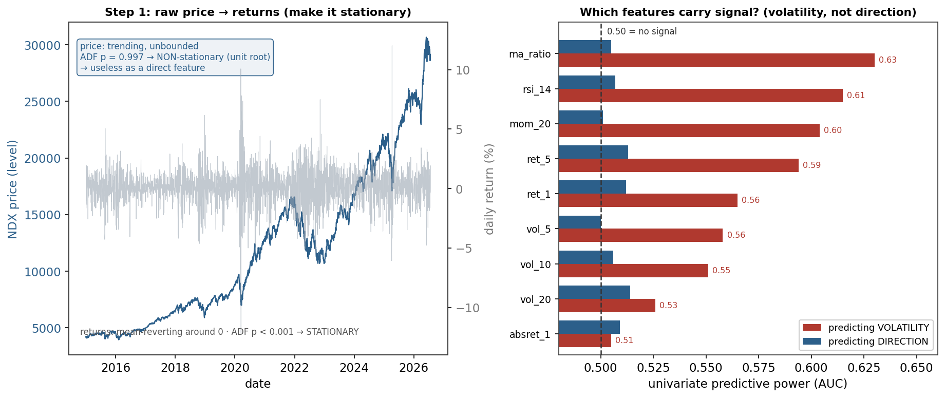
Make it stationary. Prices are non-stationary — the Nasdaq index has an augmented Dickey–Fuller p-value of 0.997, a textbook unit root — so a model fed raw prices learns the level, not the dynamics, and fails out-of-sample. The fix is to work in returns: daily returns have an ADF p-value below 0.001, firmly stationary (the left panel). Everything else is built on returns, not prices.

From there the standard families:

• Lags — past returns at several horizons (yesterday’s return, the 5- and 20-day momentum), capturing short-term reversal and longer momentum.
• Rolling statistics — realised volatility (rolling standard deviation), moving averages, and z-scores of price against its average.
• Technical indicators — RSI, MACD, Bollinger bands: compact summaries of recent price action.
• Cross-sectional — ranks or z-scores relative to the universe, so a feature means “extreme versus peers today”, not versus its own history.
• Calendar — day-of-week, turn-of-month, and other seasonal effects.

Two disciplines separate professional features from naive ones. The stationarity–memory trade-off: fully differencing a series (price → return) achieves stationarity but erases most of its memory; López de Prado’s fractional differencing takes the minimum differencing needed for stationarity while preserving as much long-memory predictive structure as possible. And scaling: standardise features, but fit the scaler on the training data only — fitting it on the whole sample leaks future distribution information backward, a mistake the data-leakage entry treats in full.

Left: the Nasdaq price is non-stationary (ADF p = 0.997, a unit root) — useless as a direct feature — while its returns are stationary (ADF p < 0.001), the foundation every other feature is built on. Right: the univariate predictive power (AUC) of nine engineered features for two targets. Every feature is essentially 0.50 for next-day direction (no signal), while several reach 0.60–0.63 for next-day volatility — the craft extracts the signal that exists and cannot manufacture the one that doesn’t.

5. What are its strengths?

• The dominant lever. Better features beat a better model almost every time; it is where effort compounds.
• Encodes domain knowledge cheaply. A volatility or regime feature injects real market understanding no generic model would discover.
• Interpretable and transferable. A good feature set is legible and works across models, a durable asset rather than a one-off fit.
• Turns non-stationary data usable. The right transforms are what make market data learnable at all.

6. What are its weaknesses?

• Look-ahead leakage. The easiest and most damaging error — a window centred on the prediction point, full-sample scaling, or revised data — makes a useless model look brilliant in backtest.
• Feature mining overfits. Try a thousand features and some will look predictive by pure chance; without multiple-testing discipline you select noise.
• Regime shift breaks features. A feature’s relationship to the target can decay or invert when the market changes — stationarity is only ever approximate.
• Labour-intensive and skill-dependent. Good features need domain insight and careful construction; garbage in, garbage out.

7. How could it apply to markets?

Directly — this is the market application, and the right panel is the honest verdict. I built nine standard features from Nasdaq history — lagged returns, multi-horizon momentum, rolling volatilities, a moving-average ratio, RSI — all strictly point-in-time, and measured each one’s univariate predictive power for two next-day targets. For direction, every single feature lands at an AUC of about 0.50 — no signal, from any of them. For volatility, several are genuinely predictive: the moving-average ratio reaches 0.63, RSI 0.61, 20-day momentum 0.60. Notably it is the trend and mean-reversion features that best forecast volatility, not the volatility features themselves — they are picking up the leverage effect, the tendency of volatility to rise after prices fall. This is the site’s thesis expressed at the level of the inputs: careful feature engineering extracts the real signal (volatility, and the structure around it) and cannot conjure the absent one (direction). The craft’s job is to build the most informative possible representation — and to be honest about which target that representation can actually serve.

8. What does the Python code look like?

import pandas as pd

def make_features(px: pd.Series) -> pd.DataFrame:
    r = px.pct_change()                                  # STATIONARITY first: prices -> returns
    F = pd.DataFrame(index=px.index)
    F["ret_1"]   = r.shift(1)                             # every feature .shift(1): point-in-time
    F["mom_20"]  = px.pct_change(20).shift(1)             # only info available at prediction time
    F["vol_10"]  = r.rolling(10).std().shift(1)           # realised volatility
    F["ma_ratio"]= (px / px.rolling(20).mean() - 1).shift(1)
    return F

# target is the FUTURE; features are the PAST — never let them overlap
y = (px.pct_change().shift(-1) > 0).astype(int)          # next-day direction
# scale AFTER splitting: StandardScaler().fit(X_train)  — never fit on the full sample

The single most important habit is the .shift(1) on every feature and the .shift(-1) on the target: features use only the past, the target is strictly the future, and they never overlap. That discipline — not the choice of indicator — is what separates a real signal from a leaked one.

9. How would I explain it to a supervisor?

“Feature engineering is turning raw prices into model-ready predictors, and it matters more than the model choice. The first and most important step is stationarity: prices have a unit root — the Nasdaq’s ADF p-value is 0.997 — so you work in returns, which are stationary at p below 0.001, and build lags, rolling volatilities, momentum, and technical indicators on top, always point-in-time with no look-ahead. The professional details are the stationarity-versus-memory trade-off, which fractional differencing handles, and scaling only on training data. On the Nasdaq I measured each feature’s predictive power honestly: every feature is 0.50 AUC for next-day direction, but several reach 0.60 to 0.63 for volatility, with trend features capturing the leverage effect. So good features extract the volatility signal that’s really there and can’t manufacture a direction signal that isn’t — and the biggest risk in the whole exercise is leaking the future into a feature.”

Nasdaq-100 index from the same multi_daily.csv as the earlier entries. Stationarity via the augmented Dickey–Fuller test (statsmodels); nine point-in-time features built with pandas; predictive power is the univariate ROC-AUC of each feature against next-day direction and next-day above-median volatility (2,883 observations), reported symmetrically so 0.50 means no signal. This begins the quant-specific ML section. Every number was checked.