Markov-Switching Regression
When the relationship itself has regimes — a regression whose coefficients switch with a hidden Markov state
The change-point detector answers when a regime changed and the HMM answers which regime we are in — but neither says what the market’s relationships become once the regime turns. That is the gap this entry closes, and it is the bridge I promised the previous one: from “a regime changed” to “so the return dynamics are now these.” A Markov-switching regression (Hamilton 1989) is an ordinary regression whose coefficients switch between a small number of hidden states that follow a Markov chain — the intercept, the slopes, and the error variance can each take different values in each regime, and the regime is inferred from the data. Fit to the beta of a defensive stock on the Nasdaq, it recovers a fact every risk manager fears and few models encode: that beta is not a constant but roughly doubles in the turbulent regime — the “diversification fails exactly when you need it” effect, turned from a warning into an estimated parameter the proposal’s Regime Agent can hand downstream.
1. What problem does it solve?
Modelling a relationship that is not stable across regimes. Standard regression assumes one set of coefficients for all time; but a factor beta, a hedge ratio, a mean-reversion speed, or a lead–lag relationship can be one thing in calm markets and quite another in a crisis. A Markov-switching regression lets the coefficients take regime-dependent values and simultaneously infers, for every day, the probability of being in each regime — so it answers two coupled questions at once: what are the dynamics in each regime, and which regime are we in now? It is the tool for the empirical fact that markets do not merely get more volatile in a crisis — the relationships between assets change.
2. What is a Markov-switching regression?
For a hidden state s_t \in \{1,\dots,K\} the model is a regression whose parameters are indexed by the state:
y_t \;=\; \alpha_{s_t} \;+\; \beta_{s_t}\, x_t \;+\; \varepsilon_t, \qquad \varepsilon_t \sim \mathcal{N}(0,\ \sigma_{s_t}^2),
and the state evolves as a Markov chain, \Pr(s_t = j \mid s_{t-1} = i) = p_{ij}. Everything that can carry a regime subscript — intercept \alpha, slope \beta, variance \sigma^2 — is allowed to switch. The crucial contrast is with the hidden Markov model already in this library: an HMM switches the marginal distribution of returns (their mean and volatility per regime), whereas a switching regression switches a conditional relationship — how y responds to x. In fact the HMM is the special case of this model with no regressor (\beta \equiv 0, only the intercept and variance switching), so Markov-switching regression is the strict generalisation: it keeps the HMM’s regime machinery and adds switching structure on top. That is exactly the extra content the Regime Agent needs — not just “how volatile is it?” but “what is the beta right now?”
3. How is it fit?
The regime is latent, so the likelihood must integrate over every possible regime path — done efficiently by the Hamilton filter, the direct analogue of the forward algorithm: carry a probability over the current regime, predict it one step through the transition matrix, reweight it by how well each regime’s regression explains today’s (x_t, y_t), and accumulate the log-likelihood. Maximising that likelihood (by EM or direct optimisation) yields the regime-specific coefficients and the transition matrix; a backward smoothing pass then gives \Pr(s_t \mid \text{all data}), the probability the figure plots. One identification wrinkle matters and is handled explicitly: the regime labels are arbitrary (nothing distinguishes “regime 1” from “regime 2” a priori — label switching), so I fix the convention by ordering regimes by fitted variance, calm before turbulent, everywhere below.
4. What did the demonstration show?
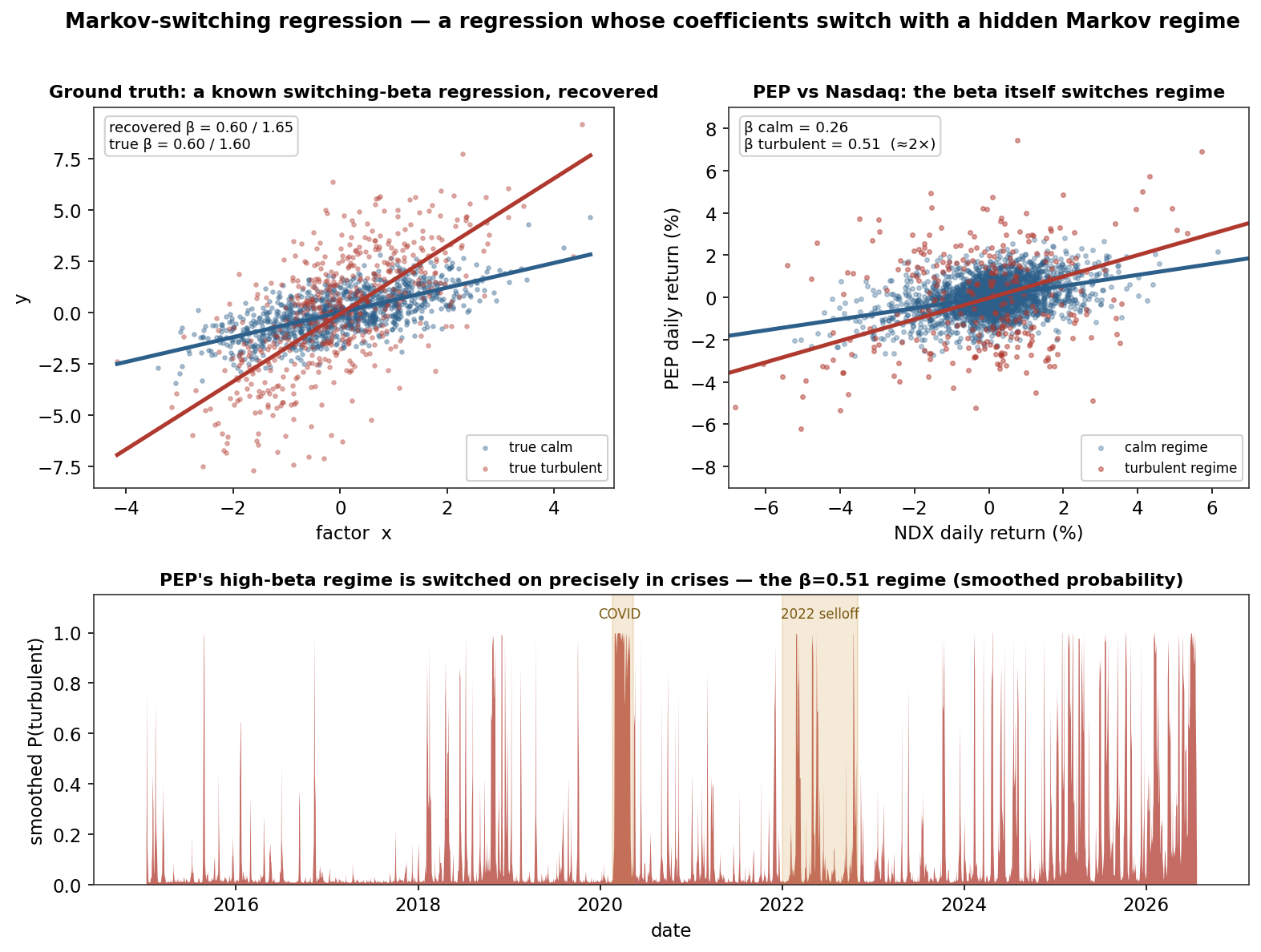
Ground truth first, the discipline this whole tier keeps. I simulated 6,000 observations from a known two-state switching-beta model — calm \beta = 0.60, turbulent \beta = 1.60, with switching variance and a known transition matrix — and fit it blind. Recovery is essentially exact: \beta =
0.60 / 1.65 against the true 0.60 / 1.60, intercepts 0.01 / {-0.06} against 0.00 / {-0.05}, volatilities 0.79 / 2.21 against 0.80 / 2.20, and regime persistences 0.979 / 0.958 against 0.980 / 0.960 (left panel). As a second, independent check on the machinery — not just its optimum — I re-implemented the Hamilton filter from scratch and evaluated the log-likelihood at the fitted parameters: it reproduced statsmodels’ value to twelve decimal places (\Delta = 2\times10^{-12}). The estimator recovers known truth, and its likelihood is exactly what it claims.
Then the market. Regressing each stock’s daily return on the Nasdaq-100’s with a two-state switching beta (2015–2026), the headline is PEP — a defensive consumer staple. Its beta is 0.26 in the calm regime and 0.51 in the turbulent one: it doubles (centre panel), and the turbulent regime is switched on precisely when it should be — smoothed probability 0.86 through the COVID crash versus 0.06 in calm 2019 (right panel). The cross-section sharpens the point rather than muddying it: NVDA jumps most in absolute terms (1.54 \to 2.08), AAPL modestly (0.96 \to 1.09), while MSFT’s beta is essentially regime-invariant (1.00 \to 1.00). Correlations converge in a crisis — but how much is an asset-specific, estimable number, not a slogan.
5. What are its strengths?
- It models switching relationships, not just switching noise. Betas, hedge ratios, and lead–lags become regime-dependent parameters — the empirical reality an unconditional regression denies.
- A generalisation of the HMM. It keeps the regime machinery this library already uses and adds conditional structure, so nothing is lost and switching coefficients are gained.
- Probabilistic regime inference for free. The same fit yields, for every day, the probability of each regime — directly usable as a soft feature.
- Interpretable. Two betas and a transition matrix are numbers a risk committee can read, unlike a black-box regime detector.
- Verifiable. As here, it recovers known coefficients on simulated data, and its likelihood can be checked independently — trustworthy before deployment.
6. What are its weaknesses?
- Smoothed probabilities use the future. The clean regime path in the figure is two-sided (it conditions on all data); a live system must use the filtered (one-sided) probability, which is noisier and lagged — precisely why online change-point detection complements it.
- The number of regimes is a choice. Two is an assumption; too few blurs distinct states, too many overfits and invites label instability.
- Linear-Gaussian within a regime. Each state is an ordinary regression; genuinely non-linear or fat-tailed within-regime behaviour is only approximated.
- Latent-state estimation is sample-hungry and can be fragile. Rare regimes (the turbulent one is ~15% of days here) are estimated from little data, so their coefficients are the least certain — visible in the turbulent beta’s wider sampling error.
- Label switching and local optima. The likelihood is multimodal; identification needs an ordering convention and good starts, or the fit is not reproducible.
7. How could it apply to markets?
This is the proposal’s Regime Agent upgraded from a labeller to a dynamics model. The HMM says which regime; change-point detection says a regime just changed; a Markov-switching regression says what the relationships have become — the regime-conditional betas, hedge ratios and factor loadings the RL Trading Agent and the Risk Agent should actually use. The PEP result is the argument in miniature: a single unconditional beta — dominated by the 85% of days that are calm — sits near 0.26 and so systematically understates the exposure in the exact regime where losses cluster, when the true beta is 0.51. A hedge or a risk limit built on that one number is wrong-footed precisely when it matters; a regime-conditional beta is not. The honest caveats shape the design rather than dent it: because the deployable signal is the filtered (one-sided) probability, the Regime Agent pairs this model’s regime-conditional parameters with the online detector’s real-time alarm; and because rare regimes are data-starved, the switching coefficients are treated as estimates with error, not constants. As always, the machinery earned trust by recovering a known model before it was pointed at real prices.
8. What does the Python code look like?
import numpy as np
from statsmodels.tsa.regime_switching.markov_regression import MarkovRegression

# y, x: stock and market daily returns (%).  Two regimes; intercept, slope AND variance switch.
mod = MarkovRegression(y, k_regimes=2, exog=x, switching_variance=True)   # switching_exog defaults True
res = mod.fit()

p    = dict(zip(res.model.param_names, np.asarray(res.params)))
var  = np.array([p['sigma2[0]'], p['sigma2[1]']])
calm, turb = np.argsort(var)                       # fix label switching: order by variance
beta = np.array([p['x1[0]'], p['x1[1]']])
print(f"beta  calm {beta[calm]:.2f}   turbulent {beta[turb]:.2f}")   # PEP -> 0.26 vs 0.51

# smoothed P(regime); for LIVE use take filtered_marginal_probabilities instead (one-sided)
p_turb = np.asarray(res.smoothed_marginal_probabilities)[:, turb]
The Hamilton filter underneath is the whole engine — carry a regime probability, push it through the transition matrix, reweight by each regime’s Gaussian regression density, normalise, and sum the logs. Re-implementing it independently and matching the library’s log-likelihood to twelve decimals is what lets me trust the parameters it returns.
9. How would I explain it to a supervisor?
“A Markov-switching regression is an ordinary regression whose coefficients switch between hidden states that follow a Markov chain. It generalises my HMM: the HMM switches the distribution of returns, this switches a relationship — so it answers what the beta or hedge ratio actually is in each regime, and infers which regime we’re in. I validated it against ground truth: I simulated data from a known switching-beta model with calm beta 0.6 and turbulent beta 1.6 and recovered 0.60 and 1.65, with the variances and transition matrix essentially exact, and I checked the estimator by re-coding the Hamilton filter from scratch — it reproduced the library’s log-likelihood to twelve decimals. On real data I regressed a defensive stock, Pepsi, on the Nasdaq: its beta is 0.26 in the calm regime and 0.51 in the turbulent one — it doubles — and that turbulent regime lights up exactly in the crises, 0.86 probability through COVID versus 0.06 in calm 2019. The cross-section is the real finding: Nvidia’s beta jumps most in absolute terms, Microsoft’s barely moves — correlations converge in a crisis, but how much is asset-specific and estimable. For my proposal this turns the Regime Agent from a labeller into a dynamics model: it supplies the regime-conditional betas the trading and risk agents should use, because a single unconditional beta understates exposure in exactly the regime where it’s dangerous. The one caveat that shapes the design is that the clean regime path uses future data — smoothed probabilities — so live I use the filtered one-sided probability and lean on my online change-point detector for the real-time alarm.”
Model: two-state Markov-switching regression (statsmodels MarkovRegression, switching intercept, slope and variance), regimes ordered by fitted variance (calm, turbulent). Ground truth: 6,000 simulated points, true \beta = 0.60/1.60, \alpha = 0.00/{-}0.05, \sigma = 0.80/2.20, transition stay-probs 0.98/0.96; recovered \beta = 0.60/1.65, \alpha = 0.01/{-}0.06, \sigma = 0.79/2.21, stay-probs 0.979/0.958. Independent Hamilton-filter log-likelihood matched statsmodels to \Delta = 2\times
10^{-12}. Real data: daily returns (%), each stock on NDX, 2015-01-05 → 2026-07-22, n = 2{,}903. Switching betas — PEP 0.26/0.51, NVDA 1.54/2.08, AAPL 0.96/1.09, MSFT 1.00/1.00; PEP turbulent resid-vol 2.19 vs calm 0.76, stay-probs 0.953/0.728, \Pr(\text{turbulent}) 0.86 (COVID) / 0.06 (calm 2019) / 0.15 (overall). Every number was checked.