Policy Gradients & Actor-Critic

Learning the policy directly — continuous actions, the score-function trick, and why baselines matter

Policy-gradient methods optimise the policy itself by gradient ascent on expected reward, handling continuous actions natively. A Gaussian-policy actor-critic learns the analytically optimal exposure on the regime environment, and the baseline’s variance reduction is measured: 3,176×.

Q-learning ended on its structural limit: the \arg\max_a needs a finite action set, but a real position is a continuous number. Policy-gradient methods remove the detour through values entirely: parameterise the policy itself — here, a Gaussian over exposure — and improve it by gradient ascent on expected reward. The result is the family that handles continuous actions natively, learns stochastic policies, and leads directly to PPO. And once again the demonstration comes with ground truth: for a mean–variance reward the optimal continuous exposure has a closed form, so the learner can be checked against the exact answer — which it hits, including a detail nobody told it: the optimal short.

1. What problem does it solve?

Direct policy optimisation: find the parameters \theta of a policy \pi_\theta(a \mid s) that maximise expected return J(\theta), without needing a value table and an argmax. This is the natural formulation when actions are continuous (position size, exposure, order rate), when a stochastic policy is wanted (exploration built in, no separate ε-greedy), or when the policy is simpler than the value function. It trades Q-learning’s off-policy convenience for directness: learn what to do, not what everything is worth.

2. What is the policy-gradient theorem?

The obstacle is that J(\theta) is an expectation over trajectories the policy itself generates — differentiating through the sampling seems impossible. The score-function (log-derivative) trick solves it:

\nabla_\theta J(\theta) \;=\; \mathbb{E}\Big[\, \nabla_\theta \log \pi_\theta(a_t \mid s_t)\; G_t \,\Big],

where G_t is the return from t. In words: increase the log-probability of actions in proportion to how well things went afterwards. No gradient of the environment is needed — only the gradient of your own policy’s log-probability, which you chose and can differentiate. Sampling this expectation gives REINFORCE: an unbiased but noisy estimator of the true gradient.

3. Why baselines — and what actor-critic adds

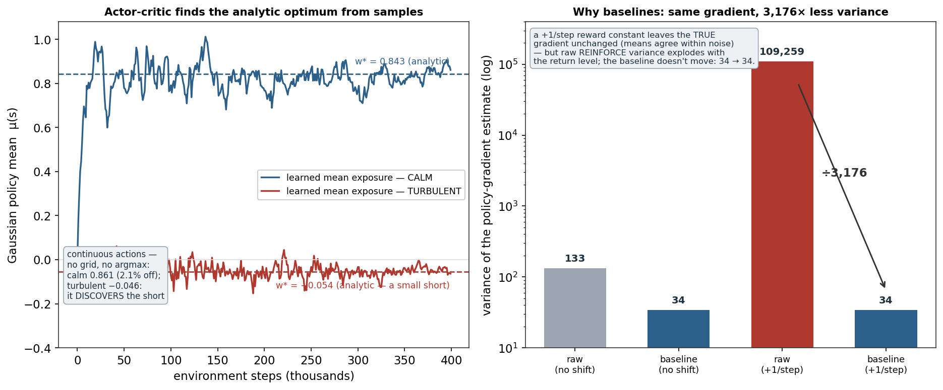
REINFORCE’s flaw is variance. Subtracting any state-dependent baseline b(s_t) from G_t leaves the gradient unbiased (the score has zero mean) but can slash its variance — and the demonstration quantifies just how much. Adding a constant +1 per step to the rewards provably does not change the true gradient; yet it blows the raw REINFORCE estimator’s variance up from 133 to 109,259, while the baselined estimator is untouched at 34 — a 3,176× difference for the identical estimand (right panel; the means agree within noise, confirming unbiasedness). Any reward scale or offset the baseline can absorb, the raw estimator pays for in variance.

The best baseline is (approximately) the state value V(s), making the weight the advantage A(s,a) = G - V(s) — how much better this action was than average. Learn V with a second model and update it by TD, and you have actor-critic: the actor \pi_\theta adjusts action probabilities using the TD error \delta = r + \gamma V(s') - V(s) as a one-sample advantage estimate, while the critic V learns to judge states — the same bootstrapping machinery as Q-learning, now in service of variance reduction.

4. What did the demonstration show?

The environment is the regime setting once more — HMM dynamics, mean–variance reward — but with unbounded continuous exposure, so the optimum is analytic: w^*(s) = \mu_s / (2\lambda\sigma_s^2), giving w^* = 0.843 in the calm regime and w^* = -0.054 in the turbulent one (yes: the risk-adjusted optimum in a negative-drift regime is a small short). A Gaussian-policy actor-critic — per-regime mean, TD critic, score-function updates — learns from samples alone: calm 0.861 (2.1% from the analytic optimum) and turbulent −0.046, sign and magnitude of the short discovered, not designed (left panel).

Left: the Gaussian policy’s mean exposure per regime over training, converging onto the analytic optima (dashed) — including the small optimal short in the turbulent regime. Right: the variance of the policy-gradient estimate. A +1-per-step reward constant leaves the true gradient unchanged but explodes the raw REINFORCE estimator’s variance from 133 to 109,259; with a value baseline it is invariant at 34 — a 3,176× reduction for the same unbiased gradient.

Getting there surfaced an honest implementation lesson, recorded because it generalises: a first attempt that clipped actions to [0,1] while computing the score on the unclipped Gaussian diverged (the mean ran to 5.6) — the score no longer matched the distribution that produced the rewards. Policy-gradient estimators are only unbiased for the exact sampling distribution you differentiate; break that correspondence anywhere and the “gradient” points nowhere. The fix (an unbounded action space, which the concave reward handles naturally) restored textbook convergence.

5. What are its strengths?

• Continuous actions, natively. A Gaussian policy outputs exposure as a real number — no grid, no argmax — exactly what position sizing needs.
• Stochastic policies with built-in exploration. The policy’s own randomness explores, and can remain deliberately stochastic where that is optimal.
• Direct and flexible. Any differentiable policy parameterisation works — from a two-parameter table here to a transformer.
• Unbiased gradients with controllable variance. The score-function estimator is exact in expectation; baselines and critics make it usable.
• The road to PPO. Actor-critic with advantage estimates is the chassis; PPO adds a stability constraint — the next entry.

6. What are its weaknesses?

• High variance is the default. Without baselines/critics the estimator can be uselessly noisy — the 3,176× is the size of the problem, not a curiosity.
• On-policy sample hunger. Vanilla policy gradients must gather fresh data after every update — worse than Q-learning’s replay for data efficiency, and a real cost when samples are market history.
• Local optima and step-size fragility. Ascent on a non-convex J can converge to poor policies, and too-large steps collapse performance — the instability PPO exists to fix.
• Correctness is delicate. The estimator is unbiased only for the exact distribution differentiated — as the clipping divergence showed.
• Credit assignment over long horizons. Returns mix many actions’ consequences; advantage estimation helps but does not solve it.

7. How could it apply to markets?

This is the algorithm family the PhD proposal’s RL Trading Agent actually needs: exposure is continuous, and the proposal’s action space A_t \in [-1, 1] is precisely a policy-gradient setting. The demonstration’s economics carry over directly — the learned policy is regime-conditional position sizing, and the fact that it recovered the risk-adjusted optimum (including the counterintuitive small short) from samples is the proof of concept in miniature. The practical warnings carry over too: on-policy sample hunger collides with finite market history, motivating the offline and off-policy variants the proposal leans on; reward constants and scales must be handled by baselines, not absorbed into variance; and every implementation subtlety (the clipping lesson) argues for the discipline this tier keeps applying — validate on a problem with a known answer before trusting the learner anywhere real. Stability under larger policy updates is the one missing piece; that is PPO.

8. What does the Python code look like?

import numpy as np

mu_theta = np.zeros(n_states)      # actor: Gaussian policy mean per state (sigma fixed)
V        = np.zeros(n_states)      # critic: state values
alpha_a, alpha_c, gamma, sd = 2e-3, 5e-2, 0.99, 0.15

s = env.reset()
for t in range(400_000):
    a = mu_theta[s] + sd * np.random.randn()          # sample from the policy
    r, s2 = env.step(s, a)                            # continuous exposure, no clipping
    delta = r + gamma * V[s2] - V[s]                  # TD error = advantage estimate
    V[s]        += alpha_c * delta                    # critic: learn to judge states
    mu_theta[s] += alpha_a * delta * (a - mu_theta[s]) / sd**2   # actor: score-function update
    s = s2
# the score  (a - mu)/sd**2  is  d/d mu  log N(a | mu, sd)  — differentiate YOUR policy, not the world

The actor’s update line is the policy-gradient theorem in one expression: score of the action taken, weighted by how much better than expected it turned out. In deep RL the table becomes a network and the update becomes backprop through \log \pi_\theta — same mathematics.

9. How would I explain it to a supervisor?

“Policy gradients optimise the policy directly: write the policy as a differentiable distribution over actions and ascend the gradient of expected return. The score-function trick makes that tractable — the gradient is the expectation of grad-log-probability of the action times the return — giving REINFORCE, which is unbiased but noisy. Baselines fix the noise: subtracting a state-value baseline leaves the gradient unbiased while collapsing variance — I measured it, a reward constant that doesn’t change the true gradient blew raw variance up three-thousand-fold while the baselined estimator didn’t move. Actor-critic operationalises that: a critic learns V by TD and the actor updates on the TD error as an advantage estimate. I verified the whole loop against a closed form — with a mean-variance reward the optimal continuous exposure is analytic, and my Gaussian actor-critic learned it to within two percent, including a small optimal short in the turbulent regime it was never told about. It’s the natural fit for continuous position sizing in my proposal; its weaknesses — on-policy sample hunger and step-size instability — are exactly what PPO addresses next.”

Environment: the regime setting with the fitted HMM transition matrix and mean–variance reward w\mu_s - \lambda(w\sigma_s)^2 (\lambda=0.15, \gamma=0.99), unbounded continuous exposure, so w^*(s)=\mu_s/(2\lambda\sigma_s^2) exactly. Actor-critic: per-state Gaussian mean, fixed \sigma=0.15, TD(0) critic, 400k steps. Variance experiment: 3,000 30-step rollouts under a fixed policy, gradient of the calm-state mean, with and without a state-time value baseline, with and without a +1/step reward shift; means agree within sampling error (unbiasedness), variances 133/34 (no shift) and 109,259/34 (shifted). Every number was checked.