Gradient Descent
Rolling downhill to the minimum — the algorithm that trains almost everything
The cost function drew the landscape; gradient descent is how you get to the bottom of it. When the cost has no closed-form minimum — which is almost always, once a model has more than a handful of parameters — you find the lowest point by feel: measure the slope under your feet and take a step downhill, over and over, until the ground goes flat. That is the whole algorithm, and it is what trains linear regressions, logistic regressions, and every neural network on earth.
The equation
Gradient descent updates the parameters by stepping against the gradient of the cost:
\theta \leftarrow \theta - \eta\,\nabla J(\theta)
repeated until convergence. \nabla J is the gradient (the vector of partial derivatives) and \eta is the learning rate (the step size).
What each symbol means
| Symbol | Meaning |
|---|---|
| \theta | the parameters being trained |
| \eta | the learning rate — how big a step to take |
| \nabla J(\theta) | the gradient of the cost — direction of steepest ascent |
| \leftarrow | “update to”: overwrite \theta with the right-hand side |
| J(\theta) | the cost function being minimised |
The gradient points uphill; the minus sign turns each step downhill.
Plain-English explanation
Imagine standing on the cost landscape in fog, wanting the lowest valley. You can’t see the bottom, but you can feel which way the ground slopes. Gradient descent is the obvious strategy: work out the downhill direction, take a step that way, and repeat. The “downhill direction” is the negative gradient — \nabla J points in the direction of steepest increase, so -\nabla J points steepest-decrease. Each step nudges the parameters a little that way, the cost drops, and after enough steps you settle at the bottom.
The size of each step is the learning rate \eta, and it is the make-or-break knob. Too small and you inch down forever, wasting compute. Too large and you leap clean over the valley and bounce up the far side — the cost oscillates and can explode to infinity. The figure shows both failure modes against a healthy run: the same problem with \eta too small creeps down slowly, with \eta just right drops to the minimum in a few steps, and with \eta too big diverges off the chart. Tuning \eta is most of the art of getting a model to train.
Why it matters in markets
Gradient descent matters because it is the one algorithm general enough to train everything, and markets are where its limits bite. A linear regression like CAPM has a closed-form solution — you can solve for the best \alpha and \beta with a formula (the normal equations). But that formula needs a matrix inversion, which costs on the order of p^3 for p parameters and becomes impossible once p is in the millions, as in any neural network. Gradient descent needs only the gradient and a step, so it scales to models the formula could never touch — which is exactly why deep learning runs on it.
Its two big caveats are also market-relevant. First, it only finds a local minimum: on the convex bowl of a linear model there is only one, so it finds the global best, but on the rugged non-convex landscape of a neural net it can settle in a mediocre valley — different random starts give different models. Second, on the full dataset each step is expensive, so in practice you use stochastic or mini-batch gradient descent, estimating the gradient from a small random sample of the data each step. The noise that injects is not just a cost — it helps the optimiser escape shallow local minima, one reason SGD-trained models often generalise better.
A simple worked example
Minimise J(w) = (w - 3)^2, a parabola with its minimum at w = 3. The gradient is J'(w) = 2(w - 3). Start at w = 0 with learning rate \eta = 0.1. Step one: the slope is 2(0 - 3) = -6, so w \leftarrow 0 - 0.1(-6) = 0.6. Step two: slope 2(0.6 - 3) = -4.8, w \leftarrow 0.6 + 0.48 = 1.08. Continuing: 1.46, 1.77, 2.02, \dots — each step closing 20% of the remaining gap, homing in on 3. Now try \eta = 1.1: the steps become 0 \to 6.6 \to -1.32 \to 8.18 \to -3.22 \to \dots, overshooting the minimum by more each time and diverging. Same cost, same start — only the step size changed.
Python implementation
import numpy as np

def gradient_descent(grad, theta, eta=0.1, steps=100):
    for _ in range(steps):
        theta = theta - eta * grad(theta)    # the one line that is the whole algorithm
    return theta

# fit AAPL ~ NDX by descending the mean-squared-error cost:
def grad(t):                                 # t = [alpha, beta]
    r = y - (t[0] + t[1] * x)                # residuals
    return np.array([-2 * r.mean(), -2 * (x * r).mean()])

theta = gradient_descent(grad, np.zeros(2), eta=0.1)    # -> [0.029, 1.013]
theta lands on the same \alpha, \beta the CAPM regression gives — gradient descent just reaches it by walking instead of by formula.
Manual / Excel calculation
You can run gradient descent in a spreadsheet for one parameter: put the current w in a cell, the gradient =2*(w-3) beside it, and the next w as =w - eta*gradient; fill the row down and watch the column march toward 3. Choosing \eta by trial is instructive — set it to 1.1 and the numbers fly apart, exactly as in the worked example.
Financial-market example — Nasdaq 100
Take the two-parameter cost from the cost-function entry — predicting AAPL’s daily return from the Nasdaq’s, J(\alpha, \beta) — and instead of solving it with a formula, walk down it. Starting from \alpha = \beta = 0, gradient descent climbs the slope and settles at \alpha = 0.03, \beta = 1.01: the CAPM alpha and beta, found by iteration. The left panel traces that path across the cost contours; the right panel is the lesson in one picture. With \eta = 0.10 the cost falls to the minimum in a handful of steps. With \eta = 0.02 it crawls — reaching the same minimum, but taking many times as many steps to get there. With \eta = 0.53 it diverges — the cost rockets off the chart as each step overshoots worse than the last.
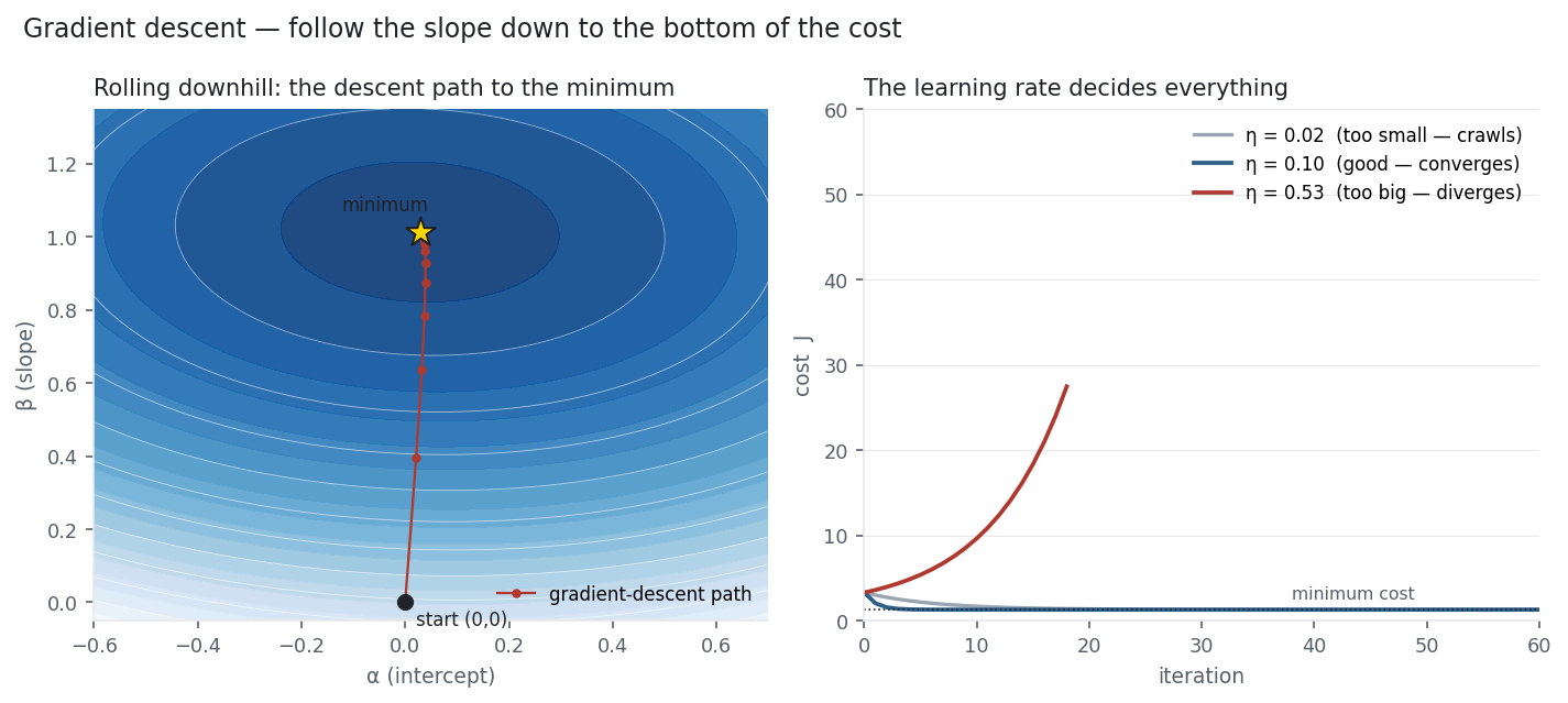
This is a well-behaved convex bowl, so any sane learning rate lands on the same answer. The reason gradient descent is worth a whole entry is what happens when the bowl becomes a mountain range — a neural network predicting returns has millions of parameters and no formula for the bottom, and then the step you take and where you start decide which valley you end up in. The algorithm is the same three symbols; the landscape is what changes.
Same multi_daily.csv as the previous entries (yfinance, adjusted closes). The descent runs on the mean-squared-error cost of AAPL daily returns regressed on NDX; the minimum matches the OLS/CAPM solution. Every number was computed and checked.
Common mistakes
- Setting the learning rate by guesswork. Too large diverges, too small wastes compute; tune it, and consider a schedule that shrinks \eta over time.
- Forgetting to scale features. Very different feature scales stretch the cost into a narrow ravine that plain gradient descent zig-zags down slowly; standardise inputs first.
- Expecting the global minimum. On a non-convex (neural-net) cost, gradient descent finds a local minimum; the start point and randomness matter.
- Using full-batch on huge data. Computing the exact gradient over millions of rows per step is wasteful; stochastic / mini-batch is the norm.
- Reading a falling training cost as done. Cost dropping means it is learning the training set — which can be overfitting; watch the validation cost.
- Ignoring the closed form when it exists. For a small linear regression the normal equations are exact and instant; gradient descent earns its keep at scale, not on toy problems.