Proximal Policy Optimisation (PPO)
A clipped objective that makes policy updates safe to repeat — the workhorse of modern RL
The policy-gradient entry ended on two named weaknesses: step-size fragility (too large a step collapses the policy) and on-policy sample hunger (each batch of experience is used once and thrown away). Proximal Policy Optimisation is the fix for both, and it is the reason PPO — not the more elegant theory around it — is the default reinforcement algorithm in practice, from robotics to the RLHF that aligns large language models. Its whole idea is a single, almost crude, modification to the objective: clip the policy update so it can never move too far from the policy that generated the data. That one change turns a fragile, one-shot gradient step into something you can safely repeat many times on the same batch — and on this library’s regime environment it converges stably to the exposure optimum we already know in closed form.
1. What problem does it solve?
Making policy-gradient learning stable and sample-efficient enough to be practical. Vanilla policy gradients demand a fresh batch of on-policy data for every small, carefully-sized update; get the step wrong and performance falls off a cliff it may never climb back. PPO lets you take many gradient steps per batch without the policy running away from the data that justified them — more learning per environment interaction, and far less sensitivity to the learning rate. For a domain where interaction is expensive or, as in markets, effectively fixed to history, that efficiency is not a nicety; it is the difference between feasible and not.
2. What is the clipped surrogate objective?
Everything hinges on the probability ratio r_t(\theta) = \pi_\theta(a_t\mid s_t) / \pi_{\theta_{\text{old}}}(a_t\mid s_t) — how much more (or less) likely the new policy is to take the action the old policy actually took. Ordinary policy gradients maximise r_t(\theta) A_t (the advantage weighted by that ratio), which is unbounded: nothing stops an update from pushing r_t to 5 or 50 on a favourable sample. PPO clips it:
L^{\text{clip}}(\theta) \;=\; \mathbb{E}\Big[\,\min\big(r_t(\theta)\,A_t,\; \text{clip}(r_t(\theta),\,1-\epsilon,\,1+\epsilon)\,A_t\big)\Big].
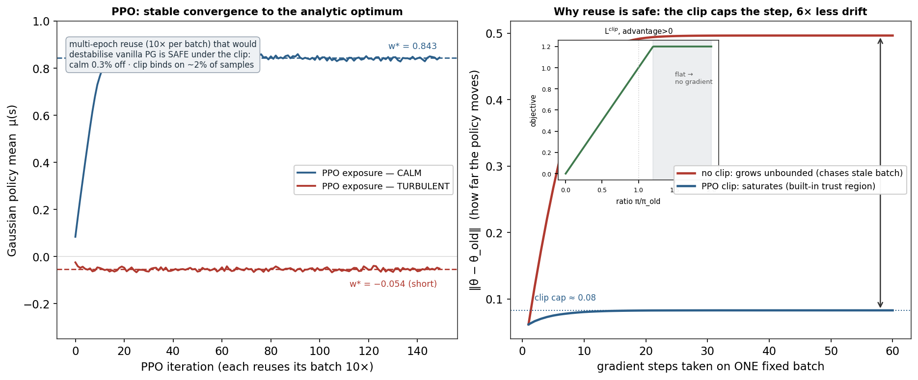
Read it through the inset in the figure. When an action was good (A_t>0), the objective rises with r_t only until r_t = 1+\epsilon (typically \epsilon = 0.2); beyond that it is flat, so its gradient is zero — the update stops rewarding you for moving further from the old policy. When an action was bad (A_t<0), the symmetric clip stops you fleeing too far. The \min makes the objective a pessimistic (lower) bound on the true improvement, so optimising it never chases an over-optimistic estimate off a cliff. It is a trust region enforced by a one-line clamp — no second-order maths, no constraint solver, which is exactly why it displaced its more principled predecessor (TRPO).
3. Why does that make sample reuse safe?
Because the clip caps how far a single batch can push the policy, no matter how many gradient steps you take on it. The right panel measures this directly: starting from one fixed batch and repeatedly updating, the unclipped objective keeps moving the policy — the update grows without bound (0.50 and still climbing) as it chases a batch whose advantages are now stale — while the clipped objective saturates almost immediately (at ~0.08), because once the ratios on the improving samples cross 1+\epsilon their gradient vanishes. A 6× difference in drift by 60 steps, and unbounded thereafter. That saturation is precisely the licence to reuse: PPO ran 10 epochs on every batch here and the clip bound on only ~2% of samples was enough to keep each iteration inside its trust region, converging cleanly where repeating vanilla updates would have diverged.
4. What did the demonstration show?
The environment is the same per-regime position-sizing problem whose optimum is analytic, w^*(s) = \mu_s / (2\lambda\sigma_s^2): 0.843 exposure in calm, −0.054 (a small short) in turbulent. A Gaussian-policy PPO agent — advantage from a value baseline, ten epochs of the clipped objective per batch — learns both from samples alone: calm 0.845 (0.3% from the exact optimum) and turbulent −0.051, converging in a few iterations and then sitting quietly on the target (left panel). The same aggressive reuse without the clip would not settle. Nothing here is approximate hand-waving: the learner hit a number computed independently in closed form, which is the validation discipline this whole tier keeps insisting on.
5. What are its strengths?
- Stable. The clip’s implicit trust region tolerates large learning rates and aggressive reuse that break vanilla policy gradients — the fragility the previous entry demonstrated, removed.
- Sample-efficient (for on-policy). Multiple epochs per batch extract far more learning per interaction — the property that matters most when data is scarce.
- Simple and robust. One clamp on the ratio; it works across enormously varied domains with little re-tuning, which is why it is the field’s default.
- General-purpose. Continuous or discrete actions, any differentiable policy — the same algorithm behind game-playing agents and instruction-tuned language models.
- Verifiable. As here, it recovers a known optimum, so its machinery can be trusted before deployment.
6. What are its weaknesses?
- Still on-policy. The clip only permits modest reuse; PPO cannot learn from arbitrary historical or off-policy data the way Q-learning can — a real limit when the only data is history.
- Heuristic, not optimal. The clip is a pragmatic surrogate for a true trust region; it can be too loose or too tight, and it has no convergence guarantee.
- Hyperparameter-sensitive in practice. \epsilon, epochs, batch size, advantage estimation (GAE’s \lambda), and reward scaling all interact — robust, not foolproof.
- Inherits policy-gradient variance. It needs good advantage estimates (a critic, GAE); a poor critic degrades it.
- No exploration guarantees. Like all policy gradients it can converge to a comfortable local optimum and stop looking.
7. How could it apply to markets?
PPO is the concrete training algorithm the PhD proposal’s RL Trading Agent would most likely use: it handles the continuous exposure actions the proposal specifies, it is stable enough to train without constant babysitting, and its sample efficiency partially eases the market-data scarcity that Q-learning’s sample hunger warned about. But its honest limit sharpens the proposal’s design rather than contradicting it: PPO is on-policy, so it cannot be turned loose to learn purely from a fixed historical archive — which is why the proposal pairs a market simulator (to generate the on-policy interaction PPO needs) with the offline and risk-constrained variants for learning from real history, and why the reward is risk-sensitive rather than raw return. The demonstration’s lesson is the reusable one: whatever the algorithm, validate it against a known optimum on a solvable version of the problem before trusting it on the market — the reinforcement-learning counterpart of a gradient check. Risk-constrained RL, which bolts hard limits onto exactly this kind of learner, is the tier’s next entry.
8. What does the Python code look like?
# PPO update on a collected batch (states, actions, advantages A, old log-probs logp_old)
for epoch in range(n_epochs):                    # REUSE the batch — the whole point
    logp  = policy.log_prob(actions, states)     # under the CURRENT policy
    ratio = (logp - logp_old).exp()              # π_new / π_old
    unclipped = ratio * A
    clipped   = ratio.clip(1 - eps, 1 + eps) * A # eps ~ 0.2: the trust region
    loss = -torch.min(unclipped, clipped).mean() # pessimistic bound -> safe to optimise
    loss.backward(); opt.step(); opt.zero_grad()
    critic_loss = (V(states) - returns).pow(2).mean()   # advantage baseline, usually via GAE
The min of the clipped and unclipped terms is the entire idea: it removes the incentive to move the policy outside the trust region, so the loop above is safe to run for many epochs on one batch — where a plain policy-gradient loop would diverge.
9. How would I explain it to a supervisor?
“PPO makes policy-gradient learning stable and sample-efficient, which is why it’s the default RL algorithm in practice. The problem it solves is that vanilla policy gradients are fragile to step size and can only use each batch once. PPO clips the ratio of new to old action probabilities inside a band around one, so the objective flattens — zero gradient — once an update tries to move the policy too far from the data that justified it. That’s a trust region enforced by a one-line clamp, and it lets you take many gradient steps per batch safely. I showed both properties on the regime sizing problem: PPO reused each batch ten times and converged to the analytic optimum, 0.3% off in the calm regime including the small short in the turbulent one, and on a fixed batch the clip saturated the update at a small cap while the unclipped version grew unbounded — a six-fold difference. Its limit for my work is that it’s still on-policy, so it needs a simulator rather than learning purely from historical data, which shapes the proposal’s design. Next is bolting hard risk constraints onto this.”
Environment: per-regime position sizing (fitted-regime means and volatilities, mean–variance reward, \lambda=0.15), where w^*(s)=\mu_s/(2\lambda\sigma_s^2) exactly (0.843 calm, −0.054 turbulent). PPO: Gaussian policy, value-baseline advantage, clip \epsilon=0.2, 10 epochs per batch, batches of 3,000; converged to (0.845, −0.051), clip binding ~2% of samples. Trust-region panel: cumulative \lVert\theta-\theta_{\text{old}}\rVert over 60 gradient steps on one fixed batch, clipped vs unclipped (0.083 vs 0.50, a 6× cap). Every number was checked.