Random Forests
Averaging many decorrelated trees — variance cancelled, overfitting tamed
The decision tree had one fatal flaw: high variance. Grow it deep and it memorises the training data; nudge the data and you get a different tree. A random forest fixes this with the simplest idea in machine learning — average a lot of them. Build hundreds of trees, each on a slightly different slice of the data and features, and let them vote. Because the errors of independent trees partly cancel, the average is far more stable than any single tree — and, crucially, without adding bias. It is the robust, low-effort default for tabular data, and on the Nasdaq it does something the earlier models couldn’t: it finds a real signal where one exists.
1. What problem does it solve?
The same classification and regression tasks as a single decision tree, but with the tree’s overfitting cured. It is an ensemble (specifically, bagging): a committee of trees whose averaged prediction generalises much better than any member. Use it wherever you’d reach for a tree but want a model you can actually trust out of sample.
2. What assumptions does it make?
The same non-assumptions as trees — nonparametric, no linearity, no scaling, axis-aligned splits — plus one that is the whole point: for averaging to reduce variance, the trees must be decorrelated. Identical trees would average to nothing gained. The forest engineers that decorrelation deliberately (below), which is what separates it from just growing the same tree many times.
3. What data does it need?
Whatever a tree needs — mixed numeric/categorical features, unscaled, with enough rows — and it scales gracefully to many features and many trees. It is particularly strong on wide, messy tabular data where linear models struggle and a single tree overfits, which describes most real-world quant feature sets.
4. How does it learn?
Two injections of randomness make the trees different from one another:
- Bagging (bootstrap aggregating). Each tree is trained on a random sample of the rows drawn with replacement — so each sees a slightly different dataset.
- Random feature subsets. At every split, each tree may only choose from a random handful of features, not all of them — which stops every tree from keying on the same dominant feature.
Then it just averages (regression) or takes a majority vote (classification). The maths of why this works is one line: if each tree has prediction variance \sigma^2 and the trees are pairwise correlated by \rho, the variance of the average of B of them is
\rho\,\sigma^2 + \frac{1-\rho}{B}\,\sigma^2.
Add enough trees and the second term vanishes, leaving \rho\sigma^2 — so the variance floor is set by how correlated the trees are. With \rho = 1 (identical trees) you gain nothing; with the random-feature trick pushing \rho down toward, say, 0.3, the average has roughly a third of a single tree’s variance. As a bonus, each bootstrap leaves ~37% of the rows unused (“out-of-bag”), which the forest scores itself on for a free validation estimate — no separate hold-out needed.
5. What are its strengths?
- Low variance, robust out of the box. Averaging tames the trees’ overfitting with almost no tuning — a superb default.
- Nonlinear, interactions, mixed data, no scaling. It inherits every convenience of trees.
- Out-of-bag validation for free. The unused bootstrap rows give an honest error estimate without a separate split.
- Feature importance. Averaged impurity reductions (or, better, permutation importance) rank the drivers.
- Parallel and forgiving. Trees train independently; it rarely breaks and rarely needs babysitting.
6. What are its weaknesses?
- Less interpretable. A single tree is a flowchart; a forest of 300 is a black box (mitigated by importances and SHAP).
- Bigger and slower. Hundreds of trees cost memory and prediction time versus one.
- Can’t extrapolate. Like any tree model, it predicts flat outside the training range.
- Biased importances. Impurity-based importance still favours high-cardinality features; cross-check with permutation.
- Not magic. It reduces variance, not bias — it can’t conjure signal that isn’t in the data (as the direction result shows).
7. How could it apply to markets?
Random forests are a genuine workhorse of tabular quant ML: combining dozens of factors and features into a signal, classifying market regimes, or ranking assets — with OOB or walk-forward validation to stay honest. And here, for the first time in this library, a model earns its keep.
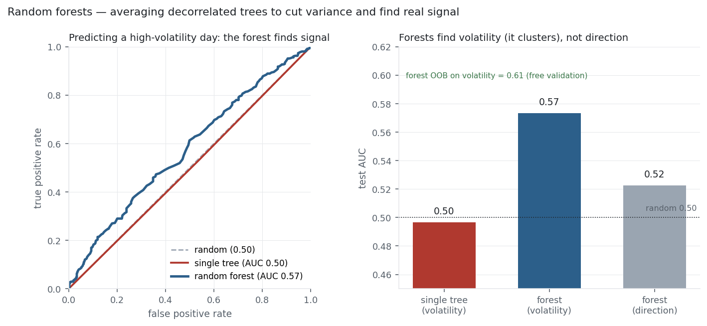
Given the last ten days’ absolute returns, a random forest predicting whether tomorrow is a high-volatility day scores a test AUC of 0.57 (and an out-of-bag AUC of 0.61) — real, repeatable skill — while a single overfit tree on the same data scores 0.50, no better than a coin flip. The ensemble extracted the volatility-clustering signal the single tree drowned in noise. But asked to predict direction — up or down — the same forest manages only AUC 0.52, barely off random. That contrast is the whole thesis of this site in one chart: volatility clusters and is forecastable, direction is essentially not, and a good model finds the first while honestly reporting the second.
8. What does the Python code look like?
from sklearn.ensemble import RandomForestClassifier
from sklearn.metrics import roc_auc_score

rf = RandomForestClassifier(n_estimators=300, max_features="sqrt",
                            oob_score=True, n_jobs=-1, random_state=0).fit(X_train, y_train)

print(rf.oob_score_)                                   # free validation from unused rows
print(roc_auc_score(y_test, rf.predict_proba(X_test)[:, 1]))   # -> 0.57 on volatility
rf.feature_importances_                                 # (cross-check with permutation_importance)
max_features="sqrt" is the random-feature-subset knob (the decorrelation lever); n_estimators just needs to be “enough” (more trees never hurt accuracy, only speed).
9. How would I explain it to a supervisor?
“A random forest averages many decision trees that are deliberately made different — each trained on a bootstrap sample of the rows and restricted to a random subset of features at each split. That decorrelation is what makes averaging work: the variance of the mean is \rho\sigma^2 + (1-\rho)\sigma^2/B, so pushing the tree-to-tree correlation \rho down collapses the variance without touching bias. It’s my robust default for tabular data, with out-of-bag error for free validation. On the Nasdaq it’s also a nice proof point: it pulls a genuine 0.57 AUC out of the volatility-clustering signal — where a single tree gets 0.50 — but stays at 0.52 on direction. It finds signal where it exists and doesn’t pretend where it doesn’t.”
Nasdaq-100 basket from the same multi_daily.csv as the Equation Library (yfinance, adjusted closes). Volatility task = classify next-day |return| above the median from the last 10 absolute returns; direction task = next-day up/down from 20 lagged returns; 70/30 time split, AUC and OOB via scikit-learn. Every number was checked.