Regime-Aware Modelling
Markets switch states — detecting regimes with a hidden Markov model, and modelling accordingly
The final entry of this library, and a synthesis of threads running through the whole of it. Again and again the same structure surfaced: K-means discovered calm and turbulent day-clusters with no labels; the Gaussian mixture modelled returns as a calm Gaussian plus a crisis Gaussian; GARCH tracked volatility persisting through time. The common thread is that a market is not one stationary process — it alternates between regimes with different means, volatilities, and correlations. A model fit to all history learns an average of regimes it will never simultaneously face, and quietly breaks when the state flips. Regime-aware modelling makes the state explicit: detect which regime you are in, and let the model — or the position size — depend on it.
1. What problem does it solve?
The non-stationarity that regime structure explains. Every validation page treated stationarity as an assumption under strain; this page models the strain directly. If returns come from two (or more) persistent states, then a single average model mis-prices both: it underestimates risk in turbulence and overestimates it in calm. Regime-aware modelling answers three questions: what states exist (their means, volatilities, durations), which state are we in now (a filtered probability, in real time), and what should change as a result (forecasts, exposures, or entire models switched by state).
2. What is the model?
The natural tool is the hidden Markov model (HMM) — and it slots exactly into this library’s sequence: an HMM is a Gaussian mixture plus a transition matrix. The GMM said each day is drawn from a calm or a crisis Gaussian but treated days as independent; the HMM adds the one missing fact — regimes persist — by making the hidden state a Markov chain. Two ingredients: per- state Gaussians (\mu_k, \sigma_k), and a transition matrix A whose diagonal is the probability of staying in a state, giving expected regime durations 1/(1-A_{kk}). Fitting is EM again (Baum–Welch — the forward-backward algorithm replacing the GMM’s independent responsibilities), and real-time inference is the forward filter: P(\text{state}_t \mid \text{data up to } t), which is point-in-time by construction — no future information.
3. What did it find on the Nasdaq?
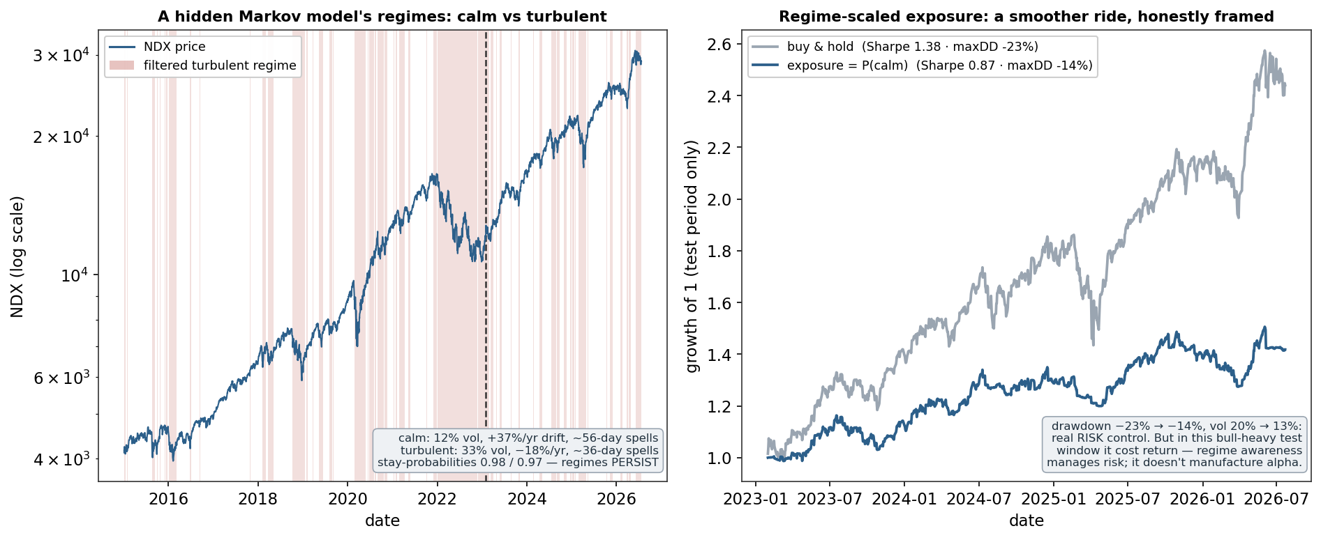
Fitting a 2-state Gaussian HMM (implemented from scratch — EM on the training 70%, parameters then frozen) recovers two sharply different worlds. A calm state: 12% annualised volatility, +37% annualised drift, spells lasting ~56 trading days on average. A turbulent state: 33% volatility, −18% drift, spells of ~36 days. The stay-probabilities are 0.982 and 0.972 — regimes are strongly persistent, which is exactly what makes them useful: knowing today’s state is informative about tomorrow’s. And the filtered turbulent periods (left panel, shaded) are not statistical abstractions — they are the late-2018 selloff, the 2020 COVID crash, the 2022 bear market, and the 2025 dip, recovered by the model from returns alone. This is the volatility-clustering thread of the entire site, now expressed as an explicit, dated state variable with measured persistence.
4. What do you do with it?
Three escalating uses. Risk awareness: the filtered P(\text{turbulent}) is a real-time dial — position sizing, VaR, and hedging can all condition on it. Regime-conditional models: fit separate models (or separate parameters) per state, so the calm model isn’t polluted by crisis dynamics and vice versa. Regime-scaled exposure: the simplest complete demonstration, run honestly here — set tomorrow’s exposure to today’s filtered P(\text{calm}), with HMM parameters fit on training data only and the filter run forward point-in-time through the test period.
The result (right panel) is the correct, nuanced verdict. The regime-scaled strategy cuts the test-period maximum drawdown from −23% to −14% and volatility from 20% to 13% — the risk control it promises, delivered. But in this particular bull-heavy test window it costs return (Sharpe 0.87 versus buy-and-hold’s 1.38): the turbulent spells it side-stepped contained V-shaped rebounds it also missed. Regime awareness manages risk; it does not manufacture alpha. That framing is this site’s thesis in one line — the volatility dimension of markets is structured and exploitable for risk, while the return dimension remains stubbornly hard.
5. What are its strengths?
- Models the non-stationarity instead of assuming it away. The single biggest mismatch between textbook ML and markets, addressed head-on.
- Persistent states are forecastable states. With stay-probabilities near 0.98, today’s regime genuinely informs tomorrow’s risk — unlike direction.
- A real-time, point-in-time dial. The forward filter uses only past data, so it can honestly drive live decisions.
- Unifies the library’s findings. K-means’ clusters, the GMM’s mixture, GARCH’s clustering — one dynamic model with dated, interpretable states.
- Genuinely useful risk control. The drawdown reduction is real and repeatable; crisis states are when correlations spike and risk models fail.
6. What are its weaknesses?
- The number of states is a choice. Two is interpretable; more states fit better but blur into each other (BIC helps, as with the GMM).
- Detection lags onset. A filter needs evidence to switch, so the first days of a new regime are misclassified — the cost is concentrated exactly at transitions.
- Regimes are a simplification. Markets don’t literally switch between two Gaussians; the states are a useful coarse-graining, not truth.
- No return edge. As the demonstration shows, knowing the risk state does not tell you tomorrow’s direction — sidestepped crashes come with sidestepped rebounds.
- Fitting subtleties. EM finds local optima, labels can switch, and parameters fit on one era may misdescribe the next — the same caveats as the GMM, inherited.
7. How could it apply to markets?
This page is the application, and its workflow generalises directly to MarketLens: run a 2–3 state HMM on returns (or on volatility features) to maintain a live filtered regime probability; display it as a risk dial; condition models on it — at minimum, evaluate every signal’s performance per regime, because a strategy that only works in calm markets needs to know when calm ends; and scale exposure or tighten risk limits as P(\text{turbulent}) rises. The honest boundary is the demonstration’s own: expect better risk-adjusted smoothness and drawdown control, not higher raw returns. Where regime-awareness pays most is defence — the 2020- and 2022-style periods where a static model, fit to the average of history, is most wrong at the worst time.
8. What does the Python code look like?
from hmmlearn.hmm import GaussianHMM
import numpy as np

X = returns.reshape(-1, 1)
hmm = GaussianHMM(n_components=2, covariance_type="full", n_iter=200)
hmm.fit(X[:split])                                   # fit on TRAIN only (point-in-time discipline)

# real-time filtered regime probability (uses only data up to t):
p_states = hmm.predict_proba(X)                      # filtered/smoothed state probabilities
p_calm   = p_states[:, np.argmin(hmm.covars_.ravel())]

exposure = np.r_[0, p_calm[:-1]]                     # tomorrow's exposure from today's filter
hmm.transmat_                                         # stay-probabilities -> expected durations
hmmlearn handles EM and filtering; the essentials are fitting on training data only, using the filtered (not smoothed) probabilities for anything tradeable, and reading the transition matrix for persistence. (The entry’s own numbers come from a from-scratch EM and forward filter — the same algorithm, verified.)
9. How would I explain it to a supervisor?
“Regime-aware modelling treats the market as switching between persistent states rather than being one stationary process. The natural tool is a hidden Markov model — exactly a Gaussian mixture plus a transition matrix, fit by EM, with a forward filter giving a point-in-time probability of each state. On the Nasdaq it recovers a calm state with 12% volatility and positive drift lasting about 56 days, and a turbulent state with 33% volatility and negative drift lasting about 36, with stay-probabilities near 0.98 — and the shaded turbulent spells are 2018, COVID, the 2022 bear, recovered from returns alone. The honest demonstration is scaling exposure by the filtered probability of calm, fit on train and filtered forward: it cuts max drawdown from 23% to 14% and volatility by a third, but costs return in a bull-heavy test window. So regime awareness is a genuine risk-management edge — persistent volatility states are forecastable — while direction stays unpredictable in every regime. It’s the whole library’s finding in one model, and where I’d take it next is evaluating every signal regime-by-regime.”
Two-state Gaussian HMM implemented from scratch (Baum–Welch EM on the first 70% of Nasdaq daily returns from the same multi_daily.csv; parameters frozen, forward filter run point-in-time thereafter). State statistics, transition matrix, durations, and the exposure-scaling comparison (Sharpe, maximum drawdown, volatility on the test period; next-day exposure from the prior day’s filtered probability) were computed and checked. This entry completes the Machine Learning Library.