Risk-Sensitive & Constrained RL
Making a learner safe — soft risk objectives, hard limits, and the shadow price of risk
Every entry in this tier so far optimised reward — and that is exactly the problem. A reward-maximising PPO agent handed the regime environment does not want a sensible position; it wants 6.3× leverage, because in a positive-drift regime more exposure means more expected return, and nothing in the objective pushes back until the account is destroyed. No trading desk — and none of the PhD proposal’s design — would let a learner behave that way. This entry adds risk to reinforcement learning in the two forms a real system needs: soft, through risk-sensitive objectives that trade return against risk continuously, and hard, through constrained MDPs that impose limits the policy cannot cross whatever the reward says. The demonstration caps that leverage-hungry agent at a defensible 1.41× with a risk budget that provably binds — the formal foundation of the proposal’s deterministic Risk Management Agent.
1. What problem does it solve?
Making reinforcement learning safe and risk-aware enough to deploy. Plain RL maximises expected return, which in markets is a recipe for ruin: it will accept enormous tail risk for a sliver of extra return, because the average reward does not see the catastrophe until it happens. Risk-sensitive and constrained RL make risk a first-class part of the problem — either woven into the objective or imposed as an inviolable limit — so the learned policy is bounded, auditable, and defensible to a risk committee rather than a liability waiting for the wrong regime.
2. Two ways to add risk
Soft — risk-sensitive objectives. Replace expected return with a risk-adjusted criterion: mean–variance (subtract \lambda\cdotvariance, the classic knob), CVaR / expected shortfall (optimise the average of the worst outcomes — the tail that actually blows up accounts), or exponential utility (a risk-aversion parameter). These express a preference: turn the knob and the policy trades return for risk continuously.
Hard — constrained MDPs. Keep the return objective but add constraints the policy must satisfy — expected cost \le budget, where the cost is CVaR, volatility, leverage, or drawdown. The agent maximises return within the feasible set; the constraint is not a preference but a rule. This is the formal shape of a risk limit, and it is what a Risk Agent enforces.
3. The soft knob, and its limitation
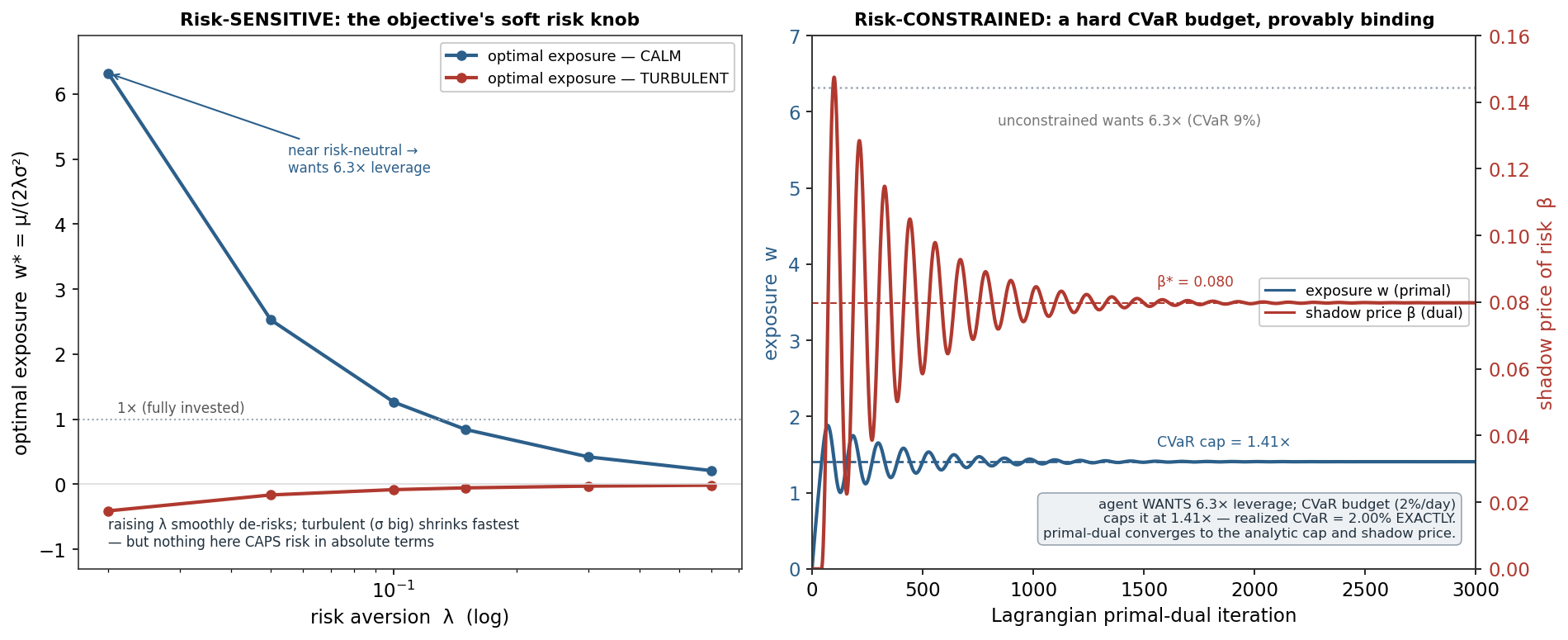
The left panel sweeps the mean–variance risk aversion \lambda, whose optimal exposure is analytic: w^*(\lambda) = \mu / (2\lambda\sigma^2). Near risk-neutral (\lambda \to 0) the agent wants 6.3× leverage in the calm regime; raising \lambda smoothly de-risks, and the turbulent regime (large \sigma) shrinks fastest — the objective already dislikes volatility. This is genuinely useful, but it carries a hidden flaw for anyone responsible for real capital: a soft objective never caps risk in absolute terms. It encodes how much you dislike risk, not a line you will not cross. Mis-tune \lambda, or meet a regime the calibration never saw, and the “risk-averse” agent can still take a position that breaches every limit you have. That gap is precisely what constraints close.
4. The hard constraint, and the shadow price of risk
A constrained MDP maximises \mathbb{E}[\text{return}] subject to \mathbb{E}[\text{cost}] \le B, and is solved by its Lagrangian:
\mathcal{L}(\pi, \beta) \;=\; \mathbb{E}[\text{return}] \;-\; \beta\big(\mathbb{E}[\text{cost}] - B\big), \qquad \beta \ge 0,
where the multiplier \beta is the shadow price of risk — the marginal return you would gain per unit of relaxed budget. The standard algorithm (PPO-Lagrangian, RCPO) is primal-dual: improve the policy on \mathcal{L} for the current \beta, and raise \beta whenever the constraint is violated (\beta \leftarrow \beta + \eta(\text{cost} - B)). At convergence the KKT conditions hold: the constraint is either slack (\beta = 0) or binds exactly (\beta > 0 and cost = B).
The right panel runs exactly this. An agent that wants 6.3× leverage (mean–variance, \lambda = 0.02) faces a hard 2%-per-day CVaR (95% expected-shortfall) budget. Primal-dual converges to an exposure of 1.407× — matching the analytic cap B / (k\sigma - \mu) to three decimals — with shadow price \beta^* = 0.080, and the realized CVaR settles at 2.00% exactly. The constraint provably binds: the leverage-hungry learner is capped at a defensible level, and the shadow price quantifies what that safety cost. A last, elegant fact ties the two halves together: this hard constraint is equivalent to a risk-sensitive objective at a specific implied risk aversion (\lambda_{\text{eff}} = 0.09) — the shadow price is simply the risk-aversion the constraint imposes on you, discovered rather than chosen.
5. What are its strengths?
- It makes RL deployable. Bounded, auditable risk is the difference between a research toy and something a desk could run.
- Hard limits are inviolable. A constraint holds regardless of reward mis-specification — a safety net against the reward-hacking that plagues RL.
- The right tail, optimised. CVaR/ES objectives target the losses that actually destroy accounts, not average-case variance.
- An interpretable price. The shadow price \beta is the marginal return per unit risk budget — a number a risk manager can reason about and set.
- A clean separation of concerns. The learner pursues return; the constraint enforces safety — exactly the actor/risk split the proposal is built on.
6. What are its weaknesses?
- Specification risk. A wrong risk measure or budget caps the wrong thing precisely; the constraint is only as good as its definition.
- Tail estimation is hard. CVaR from limited, non-stationary market data is noisy — the sample-hunger of this whole tier, concentrated in the tail.
- Primal-dual can be unstable. The multiplier oscillates before settling (visible in the figure), and poor step sizes diverge.
- Guarantees are in expectation. \mathbb{E}[\text{cost}] \le B does not prevent individual-episode breaches — real systems need hard per-step limits on top.
- It inherits RL’s fragility. Sample efficiency, stability, and stationarity problems do not disappear because risk was added.
7. How could it apply to markets?
This is the PhD proposal’s Risk Management Agent, formalised — the component that approves, scales, or rejects the RL Trading Agent’s proposed actions against hard limits on exposure, leverage, drawdown, expected shortfall, and concentration, and can override the learner regardless of what the reward suggests. The demonstration is the proof of concept in miniature: the learner’s greedy 6.3× leverage is provably capped to 1.41× by a CVaR budget, with a shadow price naming the cost. It is also the argument for why the proposal insists these controls be deterministic rather than baked softly into a reward — a soft risk penalty can be mis-tuned or gamed, but a hard constraint is a guarantee. The honest caveat sharpens the design rather than undermining it: because the Lagrangian guarantee is in expectation, a real system layers hard, deterministic, per-step limits (a maximum position, a kill-switch drawdown) on top of the risk-constrained learner — belt and braces. And as everywhere in this tier, the machinery was validated against a known optimum before being trusted with anything.
8. What does the Python code look like?
# Constrained MDP via Lagrangian primal-dual (RCPO / PPO-Lagrangian in one loop)
beta = 0.0                                        # shadow price of risk (>= 0)
for it in range(n_iters):
    # PRIMAL: improve the policy on the penalised objective  E[return] - beta * E[cost]
    #         (any RL step: PPO, actor-critic, or here the exact w* given beta)
    w = argmax_w( expected_return(w) - beta * risk_cost(w) )

    # DUAL: raise the price of risk when the budget is breached, lower it when slack
    beta = max(0.0, beta + eta * (risk_cost(w) - budget))       # eta: dual step size

# at convergence: either beta == 0 (constraint slack) or cost == budget (binds), with beta = its shadow price
The whole method is a negotiation between a return-seeking primal and a risk-pricing dual. In deep RL the argmax becomes a PPO update on the penalised advantage; the dual line is unchanged. The output is a policy that is optimal subject to the risk budget — and a shadow price that tells you what loosening the budget would buy.
9. How would I explain it to a supervisor?
“Plain RL maximises reward, which in finance is dangerous — my PPO agent wanted 6.3× leverage because more exposure meant more expected return. There are two fixes. Soft: a risk-sensitive objective like mean–variance or CVaR that trades return for risk continuously — useful, but it’s a preference, it never caps risk absolutely. Hard: a constrained MDP that maximises return subject to a risk limit it can’t cross, solved by a Lagrangian primal-dual where the multiplier is the shadow price of risk. I demonstrated the hard version against a closed form: an agent wanting 6.3× leverage under a 2%-per-day CVaR budget was driven to exactly the analytic cap of 1.41×, shadow price 0.08, with realised CVaR sitting exactly on the budget — the constraint provably binds. There’s a neat equivalence too: the hard constraint equals a risk-sensitive objective at an implied risk aversion. This is exactly my proposal’s Risk Agent — a deterministic layer that scales or rejects the trading agent’s actions against hard limits — and the reason those controls are deterministic rather than soft rewards: a constraint is a guarantee. In practice I’d still add hard per-step limits on top, because the Lagrangian guarantee is only in expectation.”
Environment: per-regime exposure with the fitted-regime means and volatilities; risk measure is the 95% CVaR (expected shortfall) of the position’s daily loss, multiplier k = \phi(z_{0.95})/0.05 = 2.063. Soft panel: mean–variance optimum w^*=\mu/(2\lambda\sigma^2) swept over \lambda. Hard panel: constrained MDP (mean–variance primal, \lambda=0.02; CVaR budget B=2\%/day) solved by Lagrangian primal-dual, converging to w=1.407 (analytic cap), \beta^*=0.080 (KKT), realised CVaR =2.00\%; implied risk aversion \lambda_{\text{eff}}=0.09. Every number was checked.