SHAP Values
Game-theoretic attribution — the unique fair split of a prediction across its features
The explainability page ended on its gap: importance and dependence are global, but the question you actually face on a given morning is local — why did the model flag today? SHAP (SHapley Additive exPlanations) is the rigorous answer. It reaches back to a 1953 result from cooperative game theory: Lloyd Shapley’s unique fair way to split a coalition’s payout among its players. Treat the features as players, the prediction as the payout, and each feature receives its Shapley value — its fair share of the prediction. The result is per-prediction attribution with a property no heuristic offers: the contributions sum exactly to the prediction minus the baseline, so every explanation is a complete, verifiable accounting.
1. What problem does it solve?
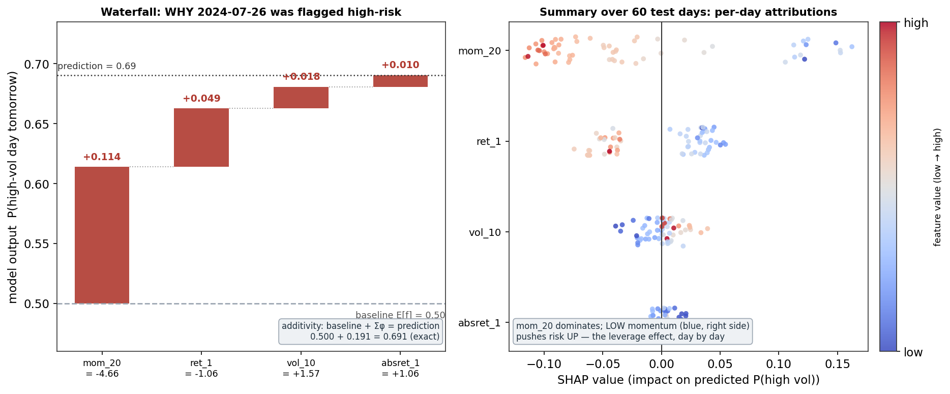
Local attribution: decomposing one specific prediction into per-feature contributions. “The model says P(high-volatility) = 0.69 tomorrow” becomes “0.50 baseline, +0.11 from the 20-day drawdown, +0.05 from yesterday’s fall, +0.02 from elevated recent vol” — an auditable account of a single output. Averaged over many predictions, the same values give a global importance ranking too, making SHAP the bridge between local and global explanation.
2. What makes it principled?
It is the unique attribution satisfying four fairness axioms. Efficiency/additivity: the contributions sum exactly to prediction minus baseline — nothing left over. Symmetry: two features that contribute identically in every context get equal credit. Dummy: a feature the model never uses gets exactly zero. Consistency: if a model changes so a feature helps more, its value cannot fall. Shapley proved these axioms pin down one formula, so SHAP is not another heuristic in a crowded field — it is the only attribution with these guarantees, which is why it became the standard.
3. What is the mechanism?
A feature’s Shapley value is its average marginal contribution across all orders of arrival. For each subset (coalition) S of the other features, compare the model’s expected output with S known versus S plus feature i known; weight and sum over every coalition:
\phi_i = \sum_{S \subseteq F \setminus \{i\}} \frac{|S|!\,(|F|-|S|-1)!}{|F|!}\,\big[v(S \cup \{i\}) - v(S)\big],
where v(S) is the expected prediction when only the features in S take the instance’s values (the rest averaged over a background dataset). The weights are exactly “average over all orderings in which the features could arrive”. The cost is the catch: 2^{|F|} coalitions, exponential in the feature count. With four features that is 16 coalitions — small enough that everything below is exact — while for large feature sets you use approximations: KernelSHAP (sampled coalitions) or, for tree ensembles, TreeSHAP, which computes exact values in polynomial time and is why SHAP is cheap for the forests and boosted models quants actually use.
4. What does it look like in practice?
The two canonical views, both on the Nasdaq volatility model. The waterfall (left) explains the single most turbulent test day, 2024-07-26: from the 0.50 baseline, the 20-day momentum of −4.7% contributes +0.114, yesterday’s −1.1% fall +0.049, elevated recent vol +0.018, and yesterday’s absolute move +0.010 — summing exactly to the 0.691 prediction. The model flagged that day overwhelmingly because the market had just fallen five percent in a month — the leverage effect, as a number, for one day. The beeswarm (right) stacks per-day attributions for 60 test days: mom_20 dominates (mean |SHAP| 0.081, twice the next feature), and its colour gradient shows the direction — low momentum (blue) sits on the positive side, pushing risk up; high momentum lowers it. The global ranking agrees with the permutation importance from the previous page, as it should — two honest methods, one answer.
5. What are its strengths?
- Axiomatically unique. The only attribution satisfying efficiency, symmetry, dummy, and consistency — not a heuristic.
- Additivity you can audit. Contributions sum exactly to prediction minus baseline (verified here to machine precision), so every explanation is complete.
- Local and global. One tool explains a single day and, averaged, ranks features overall — consistently.
- Fast where it matters. TreeSHAP makes exact values cheap for the tree ensembles that dominate tabular quant work.
- Directional detail. The beeswarm shows not just that a feature matters but how — which values push predictions which way.
6. What are its weaknesses?
- Exponential in general. Exact Shapley is 2^{|F|}; beyond small feature sets you rely on approximations with their own error.
- Correlated features again. The background-averaging (interventional) expectation creates unrealistic feature combinations when features are dependent, and credit still splits across correlated twins.
- Explains the model, not the market. SHAP faithfully attributes the model’s prediction — including its biases and overfitting; a leaked feature would get large, confident SHAP values.
- Baseline-dependent. Values are relative to the background dataset’s expectation; a different background shifts the story.
- Invites over-reading. A clean waterfall looks causal; it is a description of a correlational model, and the validation discipline still decides whether to trust the model at all.
7. How could it apply to markets?
This is the tool that turns a signal from a number into an auditable narrative — exactly what a risk committee, a client, or your own skepticism demands. On any MarketLens signal: a per-day waterfall answers “why is the model flagging tomorrow?” in economic terms (here: because the market just fell 5% — a story you can sanity-check against the leverage effect); the beeswarm gives a global check that the drivers and their directions make market sense; and sudden shifts in a feature’s SHAP distribution over time are an early warning of regime change or signal decay before it shows in P&L. The full explainability workflow, combining both pages: permutation importance for honest global ranking, partial dependence for shapes, SHAP for per-prediction accounting — with the standing caveat that a perfectly explained model can still be an overfit one, so explanation complements and never replaces validation.
8. What does the Python code look like?
import shap

model.fit(X_train, y_train)
explainer = shap.TreeExplainer(model)          # exact, polynomial-time for tree ensembles
sv = explainer(X_test)                          # shap values: (n_days, n_features)

shap.plots.waterfall(sv[i])                     # WHY did the model flag day i?
shap.plots.beeswarm(sv)                         # global summary: importance + direction
sv.values.sum(1) + sv.base_values               # == model predictions (additivity check)
TreeExplainer is the workhorse for forests/boosting; KernelExplainer handles any model by sampling coalitions. The additivity check on the last line is worth running once — it is the property that makes SHAP an accounting rather than an approximation.
9. How would I explain it to a supervisor?
“SHAP assigns each feature its Shapley value from cooperative game theory — treat features as players and the prediction as the payout, and a feature’s value is its average marginal contribution over every possible coalition of the others. It’s the unique attribution satisfying fairness axioms, and the key practical property is additivity: contributions sum exactly to the prediction minus the baseline, so each explanation is a complete accounting. I computed exact Shapley values on my volatility model — verified additivity to machine precision — and the waterfall for the most turbulent day says it was flagged because 20-day momentum was minus five percent: +0.11 of the +0.19 total, the leverage effect for a single day. The beeswarm over 60 days shows momentum dominating with low momentum pushing risk up, agreeing with permutation importance. Exact SHAP is exponential in features, but TreeSHAP makes it fast for tree models. The caveat: it explains the model, not the market — a leaked feature would get big SHAP values too — so it complements validation, never replaces it.”
Exact Shapley values (all 2^4 coalitions, interventional expectation over a 100-row training background) computed by hand for the depth-limited random forest from the explainability entry, on the same Nasdaq multi_daily.csv volatility task. Additivity verified to machine precision on both illustrated days; beeswarm over 60 random test days; mean-|SHAP| ranking cross-checked against permutation importance. Every number was checked.