Walk-Forward Validation
Train on the past, test on the future — the only honest way to backtest a temporal model
The feature engineering page ended on one rule: features must be point-in-time, using only information available at the moment of prediction. Walk-forward validation is that same rule applied to evaluation — train on the past, test on the future, roll forward, and never let the model see anything from after the point it is predicting. It sounds too obvious to state. Yet the default tool of applied ML, k-fold cross-validation, breaks it silently, and on time-series data the consequence is not a small bias but a manufactured signal: a model whose real predictive power is 0.60 can be reported at 0.87 simply because the validation leaked. This is the single most common way quant backtests lie to the people who build them.
1. What problem does it solve?
Producing an honest estimate of future, out-of-sample performance — the only number that matters for trading. Ordinary cross-validation assumes the data is independent and exchangeable, so it shuffles the rows and holds out random folds. Market data is neither: it is ordered, autocorrelated, and non-stationary. Shuffling it lets a model train on data that came after the point it tests, and when features or labels are autocorrelated it effectively trains on near-duplicates of the test points. The result is an inflated, fantasy estimate. Walk-forward validation removes the illusion by respecting the arrow of time.
2. What assumptions does it make?
That the data is ordered in time and not exchangeable, so its order must be preserved; that the future must never inform the past; and that recent history is a reasonable proxy for the near future (mild non-stationarity, which the rolling variant accommodates). It also assumes you have enough history to hold both a meaningful training window and several genuinely out-of-sample test periods.
3. What data does it need?
Any temporally ordered data — returns, features, labels. It matters most, and shuffling hurts most, when features or labels are autocorrelated or overlapping: rolling-window features, multi-day-forward labels, volatility that persists for weeks. That is exactly when adjacent rows are near-copies and a shuffled split scatters those copies across train and test.
4. How does it work?
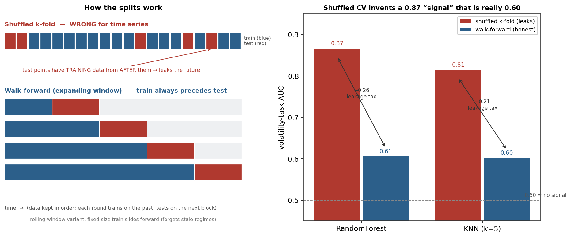
Keep the data in time order and split sequentially: train on everything up to time t, test on the block immediately after, then advance t and repeat. Two variants, shown in the left panel:
- Expanding (anchored) window — the training set grows with each step, always the full history up to t. Uses all data; assumes the distant past stays relevant.
- Rolling (sliding) window — a fixed-size training window slides forward, dropping the oldest data. Adapts to regime change and forgets stale relationships, at the cost of a shorter memory.
scikit-learn’s TimeSeriesSplit is expanding walk-forward. One refinement matters for markets and completes the picture. Even walk-forward can leak at the train/test boundary when a label spans it — an overlapping-window label at the end of training reaches into the test period. López de Prado’s fix is to purge training samples whose labels overlap the test set and to embargo a small gap after it.
The demonstration makes the stakes concrete. I built a genuinely leakage-prone but common task: predict whether the next ten days’ average absolute return is above its median — an overlapping label, since adjacent days share nine of their ten forward days. Evaluated with shuffled 5-fold CV, a random forest scores an AUC of 0.87 and a nearest-neighbour model 0.81 — apparently a strong volatility signal. Evaluated walk-forward, the same models score 0.61 and 0.60. The entire 0.21–0.26 gap is leakage: shuffling places near-identical rows — same overlapping label — on both sides of each test point, so the model recognises rather than predicts. The genuine predictability is about 0.60 (volatility is forecastable), but the shuffled 0.87 is a mirage.
5. What are its strengths?
- Honest out-of-sample estimate. It mimics live deployment — train on what you’d have had, test on what came next — so the number means something.
- Catches temporal leakage. It exposes exactly the inflation that k-fold hides, as the figure shows.
- Handles non-stationarity. The rolling variant adapts to regime change by forgetting stale data.
- The defensible standard. It is the minimum credible way to backtest any time-ordered model.
6. What are its weaknesses?
- Less data-efficient. Each point is tested at most once and the earliest data is never in a test set, so estimates use the data less fully than k-fold.
- Few, noisy estimates. A handful of sequential folds gives a higher-variance score than many shuffled ones.
- Parameter-sensitive. Window length, number of folds, and step size all affect the result.
- Still needs purge/embargo. Overlapping labels leak at the boundary unless explicitly purged.
- One historical path. Passing walk-forward is necessary but not sufficient — a single realisation can still be overfit by running many trials, which the next pages address.
7. How could it apply to markets?
This is the market discipline, not an abstraction. A backtest that shuffles time, or runs plain k-fold on a return series, is not a backtest — it is a leak, and it will hand you a strategy that evaporates in production. The demonstration quantifies precisely what is at stake: a volatility model that looks like AUC 0.87 is really 0.60, and the difference is money you would lose live. For any MarketLens signal the minimum bar is walk-forward validation — expanding or rolling, with purge and embargo whenever labels overlap — and the gap between a shuffled-CV score and a walk-forward score is the leakage tax, the amount by which your backtest is lying. The honest caveat closes the section it opens: even a clean walk-forward is a single historical path, so passing it rules out this mistake but not the deeper one of overfitting through repeated trials.
8. What does the Python code look like?
from sklearn.model_selection import TimeSeriesSplit, cross_val_score

# WRONG on time series — shuffles, leaks the future, inflates the score:
# cross_val_score(model, X, y, cv=KFold(5, shuffle=True))

# RIGHT — walk-forward: train on the past, test on the next block:
wf = TimeSeriesSplit(n_splits=5)                       # expanding window
auc = cross_val_score(model, X, y, cv=wf, scoring="roc_auc").mean()

# purge/embargo for OVERLAPPING labels (e.g. an h-day-forward target):
for train_idx, test_idx in wf.split(X):
    train_idx = train_idx[:-h]        # drop training rows whose label overlaps the test block
    model.fit(X[train_idx], y[train_idx]); ...        # then score on test_idx
The whole discipline is in not shuffling and in cutting the overlap at the boundary. TimeSeriesSplit gives you the first; the manual purge gives you the second.
9. How would I explain it to a supervisor?
“Walk-forward validation trains on the past and tests on the future, rolling forward, so the evaluation mimics live trading. The reason it’s essential is that ordinary k-fold cross-validation shuffles the data, which on a time series lets the model train on points from after the ones it tests — and with autocorrelated or overlapping labels, on near-duplicates of them — so it reports a signal that isn’t really there. I showed it: on a ten-day-forward volatility target, shuffled CV reports AUC 0.87, but honest walk-forward reveals 0.60. The 0.26 gap is pure leakage. You use an expanding or rolling window, and for overlapping labels you purge the training rows that touch the test block and embargo a gap after it. Even then it’s one historical path, so it’s necessary but not sufficient — overfitting through many trials is the next thing to guard against.”
Nasdaq-100 index from the same multi_daily.csv as the earlier entries. Task: classify whether the next ten days’ mean absolute return exceeds its trailing median (an overlapping label). AUC compared under scikit-learn KFold(shuffle=True) versus TimeSeriesSplit (expanding walk-forward), 5 folds, for a random forest and a k-nearest-neighbours pipeline (2,843 observations). Purge/embargo was also checked. Every number was verified.