Is a Factored Market State Better Than One Label?
RQ2 and H1, tested at matched cardinality — a 3×3 factored state against a flat 9-state label describing exactly the same cells
RQ2 asks whether overlapping market dimensions can be estimated more reliably than a single mutually exclusive regime label, and H1 says a multidimensional state is more stable and more useful. Both are tested here at matched cardinality, so neither model is more expressive — only cheaper. The factored state wins 5 of 9 head-to-head comparisons and loses none, which supports the second half of H1. It is more temporally stable on only 1 of 3 assets, which does not support the first. And all 18 comparisons say both descriptions are worse than using no state at all.
Research question
The PhD proposal’s RQ2 asks:
Can overlapping market dimensions be estimated more reliably than a single mutually exclusive regime label?
and H1 claims that a multidimensional state is more temporally stable and more useful than a single-label regime. Until now this was the largest untested claim in the proposal.
The question is easy to answer badly. Compare a rich factored representation against a small flat one and the factored model wins because it is bigger. Compare at equal parameter counts and the flat model loses because it has been crippled. Either way you learn about model size, not about factoring.
The design that makes it non-trivial
Compare at matched cardinality. A 3×3 factored state and a flat 9-state label describe exactly the same nine joint cells, so neither can express anything the other cannot. What differs is the price:
| joint cells | free parameters | |
|---|---|---|
| factored 3×3 — two independent chains | 9 | 24 |
| flat 9-state — one joint chain | 9 | 108 |
The flat model can represent any dependence between the two axes. The factored model assumes they evolve independently — which in markets is false, since trend and volatility are related. So the test is sharp: does the four-fold parameter saving buy more out-of-sample reliability than the misspecification costs?
That is the mechanism H1 must be claiming, and it is the only version of the claim that is not a tautology about model size.
Hypothesis
Pre-committed, following H1:
- H1-a. The factored state is more temporally stable — longer mean durations, lower flip rate — than the flat label.
- H1-b. The factored state is more useful — better calibrated forecasts than the flat label, scored the same way.
I expected both to hold, and expected the honest caveat to be that neither beats a volatility-only benchmark, because RQ1 has already shown that state information generally does not.
Data & method
Three indices — NAS100, US500, US30 — daily from 2015, roughly 1,780 scored days each after warm-up and purging.
Two observations, one per axis: daily return as a trend proxy and log realised volatility (20-day) as a volatility proxy. Volatility is modelled in logs because realised volatility is strictly positive and right-skewed, and a Gaussian emission on the raw level would put much of a state’s mass where the data cannot go.
- Factored: two independent 3-state Gaussian HMMs, one per axis.
- Flat: one 9-state Gaussian HMM on both observations jointly, diagonal covariance.
Both are refitted on a rolling window and filtered forward-only — the posterior at time t uses no data after t. That is asserted by an automated test, not by inspection: the posteriors are recomputed on a truncated series and must match to 1e-8.
Scoring reuses the RQ1 machinery exactly, so the two experiments are directly comparable: purged walk-forward logistic regression on three five-day-ahead targets, Brier score, Diebold-Mariano with Newey-West errors. Three assets × three targets = 9 head-to-head comparisons, so the deflated bar is \sqrt{2\ln 9} = 2.10.
Results
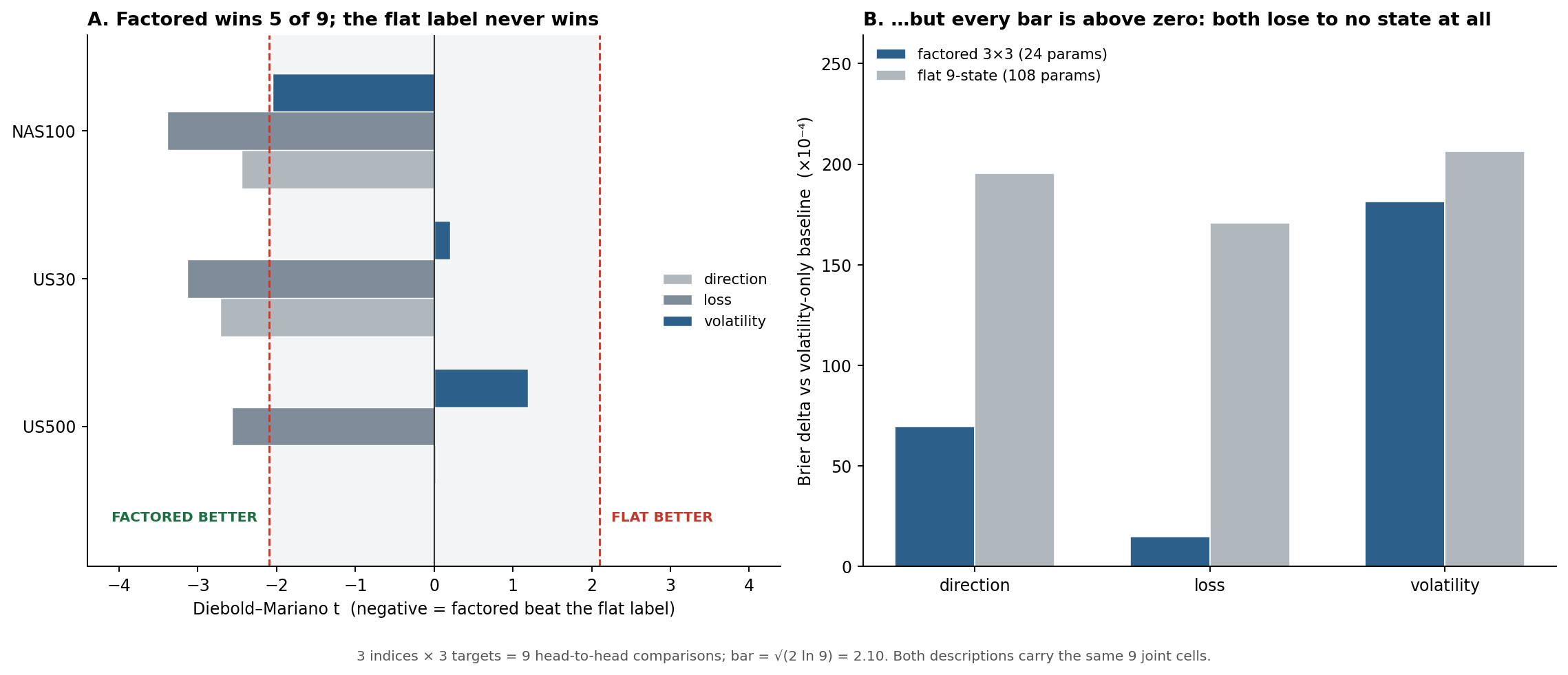
Head-to-head, the factored state wins. Of nine comparisons, five clear the deflated bar in its favour and none clears it for the flat label. It is ahead in sign on six of nine.
| t (negative = factored better) | direction | loss | volatility |
|---|---|---|---|
| NAS100 | −2.44 | −3.39 | −2.06 |
| US30 | −2.71 | −3.13 | +0.20 |
| US500 | +0.02 | −2.57 | +1.19 |
The loss target is the clean replication: factoring wins on all three assets, all three past the bar. Direction wins on two of three. Volatility is a wash.
But H1’s stability claim fails. The factored state is more persistent on NAS100 and less persistent on the other two:
| mean duration (days) | factored 3×3 | flat 9-state |
|---|---|---|
| NAS100 | 8.64 | 7.54 |
| US30 | 6.38 | 6.93 |
| US500 | 6.76 | 7.48 |
One of three is not support. Whatever advantage factoring has, temporal stability is not reliably it.
And both lose to using no state at all. In 18 of 18 comparisons the Brier score is worse than the volatility-only baseline. Averaged across the three indices:
| Brier delta vs baseline | direction | loss | volatility |
|---|---|---|---|
| factored 3×3 | +0.0069 | +0.0015 | +0.0181 |
| flat 9-state | +0.0196 | +0.0171 | +0.0206 |
Every number is positive. The factored model is consistently less costly — on the loss target it is nearly free, +0.0015 against the flat model’s +0.0171 — but “cheaper to be wrong” is not the same as right.
The verdict — and what it means for the proposal
H1-b supported, as a comparative claim. Given that you are going to describe the market with nine states, factoring them into two independent axes beats estimating one joint chain. The parameter saving outweighs the false independence assumption, and it does so consistently enough to survive a deflated bar. That is a real answer to RQ2, and it is the answer the proposal wanted.
H1-a not supported. Factoring does not reliably produce a more temporally stable state. One asset of three, and the two that disagree do so clearly.
Both are beaten by the null. This is the finding that matters most, and it is the same one RQ1 reached from a different direction: a volatility-only model with the same information beats every state description tested, factored or flat.
So RQ2’s answer is yes, and it barely matters. Factoring is the better way to build a market-state representation. It is still not a good enough reason to condition on one.
Why this is worth publishing anyway. RQ2 as written asks a comparative question — factored versus flat — and the answer is a defensible yes. But answering it exposed that the comparison sits inside a larger null. A proposal that reports only the comparative win would be technically accurate and substantively misleading. Both belong on the page.
Limitations
- Two axes, not four. The proposal’s state has trend, volatility, liquidity and structural change. This tests two. Liquidity proxies on an index are weak — Amihud on a price index is barely interpretable — so adding axes needs single-name data to be honest.
- Three correlated indices. NAS100, US500 and US30 co-move heavily, so nine comparisons are nowhere near nine independent tests, and the 2.10 bar is if anything too lenient.
- One factorisation. Trend × volatility is the obvious split, not a derived one. A different pair of axes, or a learned factorisation, could behave differently.
- Gaussian emissions, diagonal covariance. Both models share the assumption, so the comparison is fair, but neither is a good density model for daily returns.
- The flat model may be under-fitted rather than over-parameterised. 108 parameters on ~1,250 training rows is demanding; a stronger regulariser might close the gap. Testing that would be the natural follow-up.
What I learned
The design took longer than the run. My first instinct was to compare a rich factored state against a small flat one, which would have produced a clean, meaningless win — the same failure mode as measuring an overlay on raw drawdown, or scoring eight estimators on different windows. Matched cardinality is what turned a tautology into a test.
The second lesson is that a comparative result and an absolute result can point opposite ways, and reporting only one is a way of being accurate and misleading at once. Factoring genuinely beats a flat label. Neither beats doing nothing. A proposal built on the first sentence without the second would be building on sand.
NAS100, US500, US30 daily from 2015 (--offline, committed CSV), ~1,780 scored days per asset. Factored: two independent 3-state univariate Gaussian HMMs on daily return and log rv20, 24 free parameters. Flat: one 9-state bivariate Gaussian HMM with diagonal covariance on the same two observations, 108 free parameters. Both refit on a rolling 1,250-day window every 63 days and filtered forward-only; look-ahead asserted by tests/test_factored.py for both paths. Scoring: purged walk-forward logistic regression, [rv20, rv60] baseline versus baseline + posteriors, Brier at h=5, Diebold-Mariano with Newey-West lag 5. Deflated bar \sqrt{2\ln 9} = 2.10 over 9 head-to-head comparisons. Factored better past the bar: 5 of 9; flat better past the bar: 0 of 9; factored better in sign: 6 of 9. Stability: factored mean duration longer on 1 of 3 assets. Versus the volatility-only baseline: worse in 18 of 18. Code in the market-state-lab harness under src/msl/factored/.