Is a Market-State Estimate Worth Anything?
Eight state estimators, seven assets, one honest benchmark — a volatility-only model seeing the same information
RQ1 asks which methods most reliably identify market state. This experiment asks the harder question underneath: does any of them add decision value beyond a continuous volatility signal? 168 comparisons across seven assets, Diebold-Mariano tests, and a deflated bar of |t| > 3.20. State makes direction forecasts worse in 53 of 56 cases and adds no risk-adjusted value. The one apparent survivor — a simple trend rule on the volatility target — points the right way on 7 of 7 assets but clears the bar on only 2, and not on the asset it was discovered on. Meanwhile 18 comparisons are significant harms against 0.23 expected by chance.
Research question
The PhD proposal’s RQ1 asks which statistical, econometric and ML methods most reliably identify market states out of sample. Reliability, though, is not self-defining. A method can produce a stable, plausible, well-recovered state estimate that makes no difference to any decision. So this experiment tests the question underneath:
Does conditioning on a market-state estimate improve out-of-sample forecast calibration or risk control, beyond what a continuous volatility signal using the same information already provides?
That final clause is the entire design. Comparing a state-conditional model against buy-and-hold, or against nothing, would only demonstrate that volatility is informative — which nobody disputes. The benchmark here is a model that sees the same volatility features and simply does not see the state. Whatever the state adds over that, and only that, is the incremental value of state information.
Hypothesis
From the proposal’s own position, and from what this lab has already found in regime-conditioning and regime-conditional calibration:
- H-a. State information will not improve direction forecasts. Expected null.
- H-b. State information will improve volatility-regime calibration.
- H-c. A state overlay on volatility targeting will not improve risk-adjusted outcomes beyond the volatility scaler itself.
H-a and H-c are predictions of failure. Stating them in advance is what makes the result informative either way.
Data & method
Daily data for seven pre-declared assets — NAS100, US500, US30, AAPL, MSFT, JPM, XOM — from 2010 to August 2026. The single-name list is fixed and never edited to match today’s index membership, which is what keeps the panel free of survivorship bias.
Eight state estimators: three transparent baselines (moving-average crossover, trailing-return sign, EWMA slope), a Kalman local-linear-trend filter, a Gaussian HMM, a Markov-switching regression, and CUSUM and BOCPD change-point detectors. Each emits a filtered probability vector over {down, range, up}; the value at time t uses only data up to t, enforced by an automated look-ahead test rather than by inspection. The harness’s ninth estimator, a do-nothing constant, is excluded: a state that never changes carries no information to test, and scoring it would only pad the comparison count and loosen the bar.
Every method is scored on identical dates. Methods that fit parameters surrender a training window, so their usable spans are shorter than the baselines’. Scoring each against its own benchmark makes every individual comparison fair while making the ranking partly a comparison of periods. The panel is therefore aligned to the intersection of all spans — 3,401 shared dates, 2,830 scored after the purged walk-forward, identical for all 168 cells.
Calibration. Walk-forward logistic regression, purged by the label horizon, comparing [rv20, rv60] against [rv20, rv60, p_down, p_range, p_up] on three five-day-ahead targets: direction (return positive), loss (return below minus one trailing standard deviation), and volatility (realised volatility above its trailing median). Scored by Brier; a negative delta means the state helped. The estimator’s own rolling flip rate is added to both models, so the benchmark already sees how much the state has been churning.
Significance. Diebold-Mariano tests on the per-observation loss differential with Newey-West standard errors, because overlapping five-day labels make the differentials serially correlated and an i.i.d. error would manufacture significance. With 168 comparisons the relevant bar is not 1.96: under the null the largest of N t-statistics is around \sqrt{2\ln N}, so the deflated threshold is |t| > 3.20.
Risk control. Volatility targeting at 10% annualised, with and without a state overlay that multiplies exposure by (1 - p_{\text{down}}) — pre-committed, and purely defensive so that it can only ever reduce exposure. Net of 2bp costs on turnover.
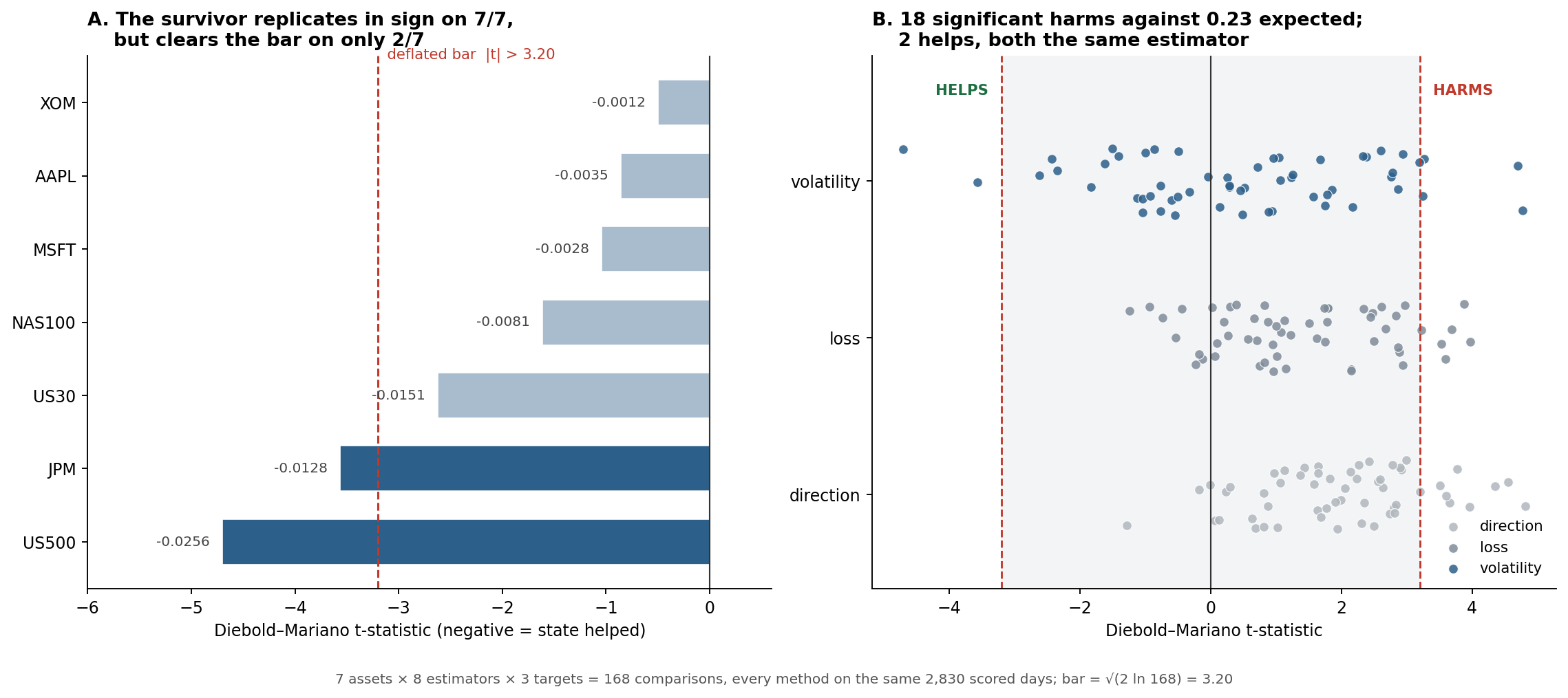
ewma_slope on the volatility target points the helpful way on all seven assets, but only US500 and JPM clear the deflated bar — and NAS100, the asset the result was discovered on, reaches only t = −1.62. Right: all 168 comparisons. The shaded band is the region where nothing can be claimed. Eighteen points sit in HARMS against 0.23 expected by chance; two sit in HELPS, both the same estimator on the same target.Results
Direction: the null is emphatic. State made direction forecasts worse in 53 of 56 asset-method pairs. Not one comparison helps at any threshold, and eight are significant harms. Whatever a market-state estimate is for, it is not timing next week’s return.
Loss: the same, slightly softer. Worse in 48 of 56, no helps, six significant harms.
Volatility regime: worse in 33 of 56, and the two helps are the whole story. Only ewma_slope clears the bar, and only on two assets:
| asset | Brier delta | t |
|---|---|---|
| US500 | −0.0256 | −4.70 |
| JPM | −0.0128 | −3.57 |
| US30 | −0.0151 | −2.62 |
| NAS100 | −0.0081 | −1.62 |
| MSFT | −0.0028 | −1.04 |
| AAPL | −0.0035 | −0.86 |
| XOM | −0.0012 | −0.50 |
The sign is negative on 7 of 7 — the effect points the same way everywhere, which is not nothing. But it reaches significance on two, and NAS100 is not one of them. That is the asset this result was originally found on, at t = −3.93 over a 2018–2026 window. Extend the sample to 2010 and it falls to t = −1.62.
Adding state can significantly hurt. Eighteen of 168 comparisons are significant harms against 0.23 expected under the null at this bar — roughly seventy-eight times chance. They cluster in ma_cross (5) and hmm_gaussian (5), and on the direction target (8). The largest are kalman_trend on XOM direction (t = +4.82) and ma_cross on XOM and NAS100 volatility (+4.78, +4.70).
Risk control: the null holds across the panel. Averaged over seven assets — buy-and-hold Sharpe 0.637, the volatility-target baseline 0.663 at 11.4% volatility, and the state overlay 0.592 at 9.1%:
| measure | overlays better than baseline, of 56 pairs |
|---|---|
| raw maximum drawdown | 44 of 56 |
| drawdown per unit of volatility | 12 of 56 |
| Sharpe ratio | 4 of 56 |
Read raw drawdown alone and the overlay looks good. That is an artefact: it can only cut exposure, so it always ends up holding less, and a rule that holds less always shows a shallower drawdown. Read risk-adjusted and it reverses — the overlay’s drawdown per unit of volatility is −2.110 against the baseline’s −1.958, and its Sharpe is lower, on higher turnover.
The verdict — and what it means for the proposal
H-a confirmed, decisively. 53 of 56 worse, zero helps, eight significant harms. State does not time returns, and on several asset-method pairs it measurably degrades the forecast.
H-b not confirmed. One estimator on one target points the right way on every asset but reaches significance on two of seven, and fails on the asset it was discovered on. The honest label is suggestive and asset-specific, not a finding.
H-c confirmed, more strongly than on one asset. The overlay improves Sharpe in 4 of 56 pairs and risk-adjusted drawdown in 12. The same de-risking is available for nothing by lowering the volatility target — no model, no turnover.
This tightens the proposal rather than flattering it. “Market-state information is a calibration and risk-control signal, not a return-timing signal” survives only in its first half, and weakly: the calibration benefit is narrow, asset-specific and not yet replicated, and the risk-control half does not hold once exposure is controlled for.
What the panel cost the headline. On one asset over one window, ewma_slope produced a 9% relative Brier improvement at t = −3.93 that survived every correction available at N = 24. Widen to seven assets and 2010–2026, and the same estimator on the same target reaches t = −1.62 on that asset. Nothing was done wrong in the first analysis. It was simply a single draw, and a single draw is what the deflated bar exists to distrust.
Limitations
- One market era, seven correlated assets. Three indices and four US large caps do not span the space of markets, and the equity names co-move. Effective sample size is well below 168 independent tests, which makes the deflated bar, if anything, too lenient.
- The DM test is slightly liberal. Its empirical size measured ~0.07 against a nominal 0.05, so borderline results deserve more scepticism than their p-values suggest.
- One overlay rule. (1 - p_{\text{down}}) is defensible and pre-committed but arbitrary; a different mapping from state to exposure could behave differently.
- Not reproducible from the committed data. This run used freshly downloaded prices to 2026-08-24, so re-running later will move the numbers. The committed CSV reproduces the single-asset version, not this one.
- Index, not total return, and no borrowing constraint on the leveraged volatility target.
What I learned
The lesson this experiment kept teaching, in three different costumes, is fix the comparison before reading the number.
First it was raw drawdown, which made every overlay look successful until exposure was controlled for. Then it was the scored window: eight methods each fairly benchmarked still produced an unfair ranking, because half were judged on a harder period than the others — and correcting it removed four “significant harms” I had already published. Then it was the asset. A result that survived multiple-testing correction on Nasdaq did not survive being asked the same question of six other assets.
None of these was a coding error. Each was a comparison that looked obviously fair and was not, and in each case the correct comparison changed the answer. That is the failure mode worth guarding against — not arithmetic, but a benchmark that quietly answers a different question.
The second lesson is what a fair benchmark costs a hypothesis. Against buy-and-hold, almost everything here would have looked like a win. Against a volatility-only model with the same information, 166 of 168 comparisons are neutral or harmful. That is the difference between a result and an artefact, and it is the standard the LLM-trading literature conspicuously fails to meet.
Seven assets (NAS100, US500, US30, AAPL, MSFT, JPM, XOM), daily, 2010 to 2026-08-24. Common window 3,401 shared dates, 2,830 scored — identical for all 168 cells via msl decision -c configs/trend_mixed.yaml --refresh --common-window. Eight estimators through the market-state-lab harness; all estimates filtered and look-ahead tested. Calibration: purged walk-forward logistic regression, [rv20, rv60] vs [rv20, rv60, p_down, p_range, p_up], plus the estimator’s own 60-day flip rate in both models. Significance: Diebold-Mariano with Newey-West lag 5; deflated bar \sqrt{2\ln 168} = 3.20. Helps: ewma_slope/volatility on US500 (−0.0256, t −4.70) and JPM (−0.0128, t −3.57); mean across seven assets −0.0099, negative on 7/7. Harms: 18 of 168 (direction 8, loss 6, volatility 4) against 0.23 expected. Direction worse in 53/56, loss in 48/56, volatility in 33/56. Risk control: 10% annualised volatility target, exposure capped at 2×, overlay (1-p_{\text{down}}), 2bp turnover cost; buy-and-hold Sharpe 0.637 / vol 23.1% / max drawdown −45.6% / dd-per-vol −2.006; baseline 0.663 / 11.4% / −22.1% / −1.958 / 7.0× turnover; overlay 0.592 / 9.1% / −18.8% / −2.110 / 8.7×. Because this run refreshed prices, the numbers are as-of 2026-08-24 rather than reproducible from the committed CSV.