Does Conditioning on Regime Actually Help?

A fair out-of-sample test of the proposal’s central hypothesis — with a result that sharpens it

H5 is the heart of the PhD proposal: that conditioning decisions on estimated market regime improves performance. This experiment tests it as fairly as I can — a real-time, no-look-ahead HMM regime against a regime-blind volatility scaler and static buy-and-hold, out-of-sample and net of costs — and finds the honest answer: regime awareness buys risk control, but the discrete regime adds nothing a volatility signal doesn’t, and no edge is statistically significant.

Research question

This is the experiment the whole PhD proposal leans on. Its central bet — hypothesis H5, and research question RQ6 — is that conditioning forecasting and decision models on estimated regime probabilities improves economic performance. Every regime entry in the library built the machinery; this experiment asks whether the machinery pays. And it asks it in the sharpest, least flattering form I could design: not “does a regime-aware strategy beat buy-and-hold?” (too easy — any de-risking rule cuts drawdown in a bull market) but “does a discrete, real-time-estimated regime beat a regime-blind volatility signal that uses the same information continuously?” If regime only ties a volatility scaler, then for the purpose of sizing a position the “regime” is just repackaged volatility, and H5’s economic claim needs rethinking.

Hypothesis

I pre-committed to a split prediction, and deliberately gave the null a real chance. H5 (proposal): regime-conditioning improves risk-adjusted performance. My honest prior: it improves risk control (drawdown) robustly — consistent with everything this site has found — but the discrete regime adds little beyond a continuous volatility signal, and any Sharpe improvement over a decade of daily data will be too small to be statistically significant. A genuine test has to be able to return that null, so I built it to.

Data & method

Daily Nasdaq-100 returns, 2015–2026 (multi_daily.csv), evaluated out-of-sample on 2016–2026 after a 252-day burn-in.

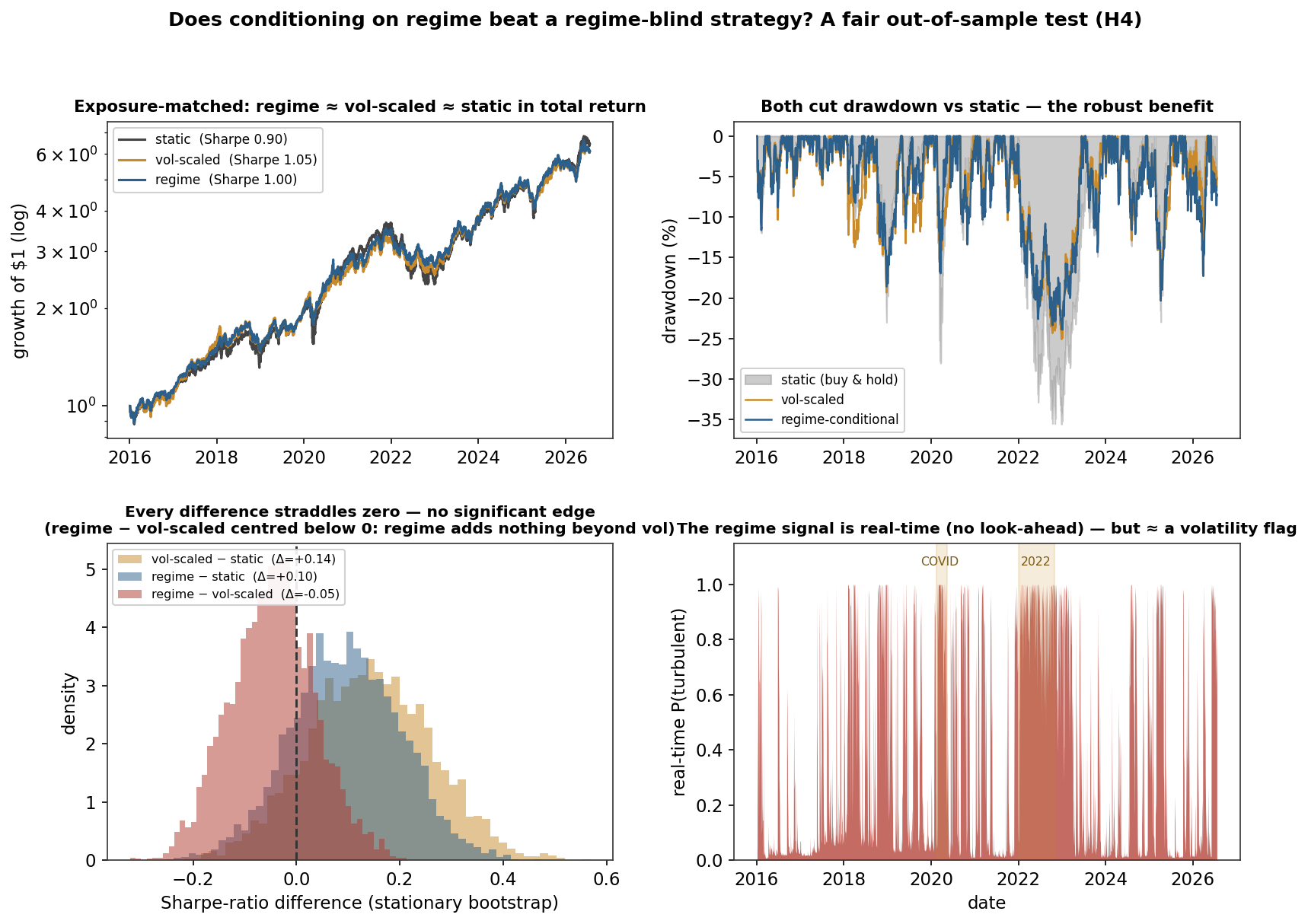
The regime is estimated in real time, with no look-ahead — the part that makes this fair. A two-state Gaussian hidden Markov model (my own Baum–Welch implementation, since the discrete regime is exactly the library’s HMM) is re-fit quarterly on an expanding window, and the regime at each day is the filtered (forward-only) probability of the high-volatility state — never the smoothed probability, which would peek at the future. The fitted states are a calm regime at 13.8% annualised volatility and a turbulent one at 34.4%; the signal flags COVID (P = 0.86) and the 2022 bear market (P = 0.98) point-in-time while staying quiet in calm 2017 (P = 0.12).

Three long-only Nasdaq strategies then use the same lagged information, differing only in how:

• Static — constant exposure (regime-blind, the baseline).
• Volatility-scaled — continuous inverse-volatility exposure, w_t \propto 1/\hat\sigma_{t} (uses volatility, but no discrete regime).
• Regime-conditional — exposure set by the estimated regime (a discrete 1.0 / 0.4 split, and a smooth version scaled by the turbulent probability).

All three are compared exposure-matched (normalised to equal average investment, so only timing differs), net of 2 bps per unit turnover. The headline metric is the annualised Sharpe ratio (scale-invariant), and — because a single backtest number means nothing without an error bar — I put a stationary bootstrap (Politis–Romano, ~20-day blocks, 4,000 resamples) confidence interval on every Sharpe difference.

Results

Both risk strategies beat static on risk-adjusted metrics. Static buy-and-hold earns a Sharpe of 0.90 with a −36% drawdown. Volatility-scaling lifts that to 1.05 with a −25% drawdown; the regime-conditional version reaches 1.00 with a −24% drawdown; Calmar improves from 0.55 to ~0.75–0.78. The drawdown panel shows why — both risk strategies ride through 2018, 2022 and the smaller selloffs well above buy-and-hold’s underwater curve. Directionally, H5 holds: conditioning on the volatility environment improves risk-adjusted outcomes.

But none of it is statistically significant, and the discrete regime adds nothing beyond volatility. This is the decisive part. Every bootstrap Sharpe-difference distribution straddles zero: volatility-scaling beats static by only +0.14 (95% CI [−0.09, +0.37], p = 0.24), regime beats static by +0.10 ([−0.11, +0.30], p = 0.36), and — the crucial comparison — regime minus volatility-scaling is −0.05 ([−0.20, +0.12], p = 0.56), a distribution centred below zero. Over a decade of daily data, the improvement from a regime-blind volatility signal is not distinguishable from noise, and the sophisticated discrete regime does not beat it. As a position-sizing device, the regime is a coarsened volatility flag.

Top-left: exposure-matched growth of $1 — static, volatility-scaled and regime-conditional are nearly indistinguishable in total return (Sharpe 0.90 / 1.05 / 1.00). Top-right: drawdown — both risk strategies cut the −36% static drawdown to about −24%, the robust benefit. Bottom-left: stationary-bootstrap Sharpe-difference distributions — all three straddle zero (no significant edge), and regime − volatility-scaled is centred below zero, so the discrete regime adds nothing beyond the volatility signal. Bottom-right: the real-time regime probability, flagging COVID and 2022 with no look-ahead, but tracking volatility so closely it is effectively a volatility flag.

The verdict — and what it means for the proposal

The honest reading is a partial null, and it is more useful to the proposal than a clean win would have been. H5’s risk claim survives — regime and volatility awareness both cut drawdown materially and robustly, exactly as this site keeps finding. But H5’s economic-outperformance claim, tested as position sizing, does not: the edge over a naive volatility scaler is negative and insignificant, and the edge over static is insignificant too. For sizing a position, a discrete regime is not worth more than a volatility number.

That is a genuine steer, not a defeat, and I would change the proposal’s framing accordingly. The Regime Agent should not be justified by regime-conditioned sizing alpha — this experiment says there isn’t any. It should be justified by the two things a volatility scaler provably cannot do, both already demonstrated elsewhere on this site: online detection of regime changes (the change-point detector is a timing alarm, not a sizing knob), and conditioning relationships on regime (the Markov-switching finding that a stock’s beta doubles in the turbulent state — something no scalar volatility target can express). The untested half of H5 — whether regime-conditioning improves probability calibration — is the other place its value may really lie, and is a natural next experiment. In short: keep the Regime Agent, but sell it on detection and relationship-conditioning, not on sizing.

Limitations

• One index, one decade, one split. The bootstrap widths already say the sample is too short to resolve a Sharpe difference of ~0.1; a longer history or a panel of assets could tighten it (or confirm the null).
• A simple regime rule. Two states, a 1.0 / 0.4 exposure map; a richer regime taxonomy or a regime-conditioned directional signal might do more — but each added degree of freedom is another chance to overfit, which is precisely the discipline the backtest-overfitting experiment warns about.
• Sizing only. This tests regime for position sizing. It does not test the two uses the verdict points to (detection timing, relationship-conditioning) or the calibration half of H5 — so it refutes the narrow claim, not the broad one.
• Costs are stylised (flat 2 bps/turnover); the discrete regime’s switching turnover would be penalised harder under realistic, volatility-dependent costs — which only strengthens the “discrete regime isn’t worth it for sizing” conclusion.

What I learned

The lesson I will carry into the thesis is that the right benchmark is everything. Measured against buy-and-hold, regime-conditioning looks like a clear win; measured against the fair benchmark — a regime-blind strategy using the same volatility information — the win evaporates. A hypothesis is only tested against the strongest alternative it must beat, and here that alternative is “just use volatility.” The second lesson is the value of an error bar: the point estimates (Sharpe +0.10 to +0.14) would have read as success in a naive backtest; the bootstrap is what turned “regime helps” into “regime helps, but not distinguishably, and not beyond volatility.” That is the difference between a finding and a story, and it is exactly the kind of result the Quant Lab exists to produce.

References

• Hamilton, J. D. (1989). A New Approach to the Economic Analysis of Nonstationary Time Series and the Business Cycle. Econometrica, 57(2).
• Ang, A., & Bekaert, G. (2002). International Asset Allocation with Regime Shifts. Review of Financial Studies, 15(4).
• Politis, D. N., & Romano, J. P. (1994). The Stationary Bootstrap. Journal of the American Statistical Association, 89(428).
• Moreira, A., & Muir, T. (2017). Volatility-Managed Portfolios. Journal of Finance, 72(4).

Regime: two-state Gaussian HMM (own Baum–Welch), re-fit quarterly on an expanding window; filtered (forward-only) turbulent probability, no look-ahead; states 13.8% / 34.4% annualised vol, turbulent fraction 0.35. Strategies exposure-matched, net of 2 bps/turnover, evaluated 2016–2026. Sharpe: static 0.90, vol-scaled 1.05, regime 1.00. Bootstrap (stationary, ~20-day blocks, 4,000 resamples) Sharpe differences: vol−static +0.14 [−0.09, +0.37]; regime−static +0.10 [−0.11, +0.30]; regime−vol −0.05 [−0.20, +0.12] — all straddle zero. Computed from equations/multi_daily.csv, verified in the sandbox.