Seven Specialists, One Dimension
The effective number of independent signals says the estimator panel is healthy. It says the same thing when seven estimators measure one quantity badly — so the count was never evidence
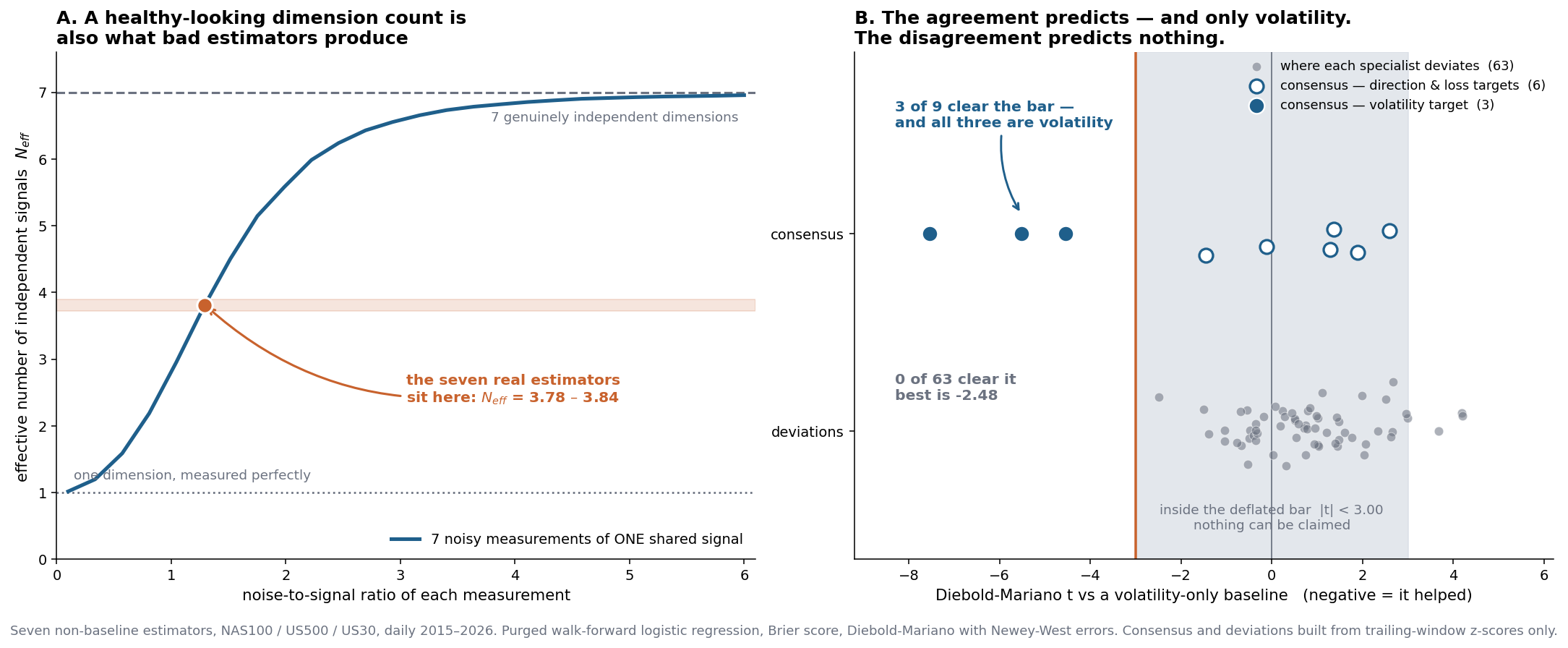
A council of specialists only works if the specialists cover different dimensions. The standard check — the effective number of independent signals — returns 3.8 of 7 here, which looks healthy. It is not evidence, because seven noisy measurements of a single quantity decorrelate exactly like seven genuine dimensions. Splitting the panel into what the estimators agree on and where each departs from it settles the question: the agreement clears the deflated bar 3 times of 9, the deviations 0 times of 63, and putting the deviations back degrades the consensus on all three assets.
The claim this tests
The proposal is built on a council: many specialist models, each covering a different dimension of market state, whose outputs are then reconciled. That architecture has a prerequisite so basic it is easy to skip — the specialists have to be looking at different things. If they all measure one quantity, their disagreement is measurement error, and every downstream mechanism that trades on disagreement is aggregating noise.
So before adding an eighth estimator, it is worth asking whether the seven already built span more than one dimension.
The check that looks sufficient and is not
The standard diagnostic is the effective number of independent signals, from the dispersion of the correlation matrix’s eigenvalues:
N_{\text{eff}} = \frac{\left(\sum_i \lambda_i\right)^2}{\sum_i \lambda_i^2}
It returns 1 when every signal is a copy of every other, and M when they are orthogonal. On the seven non-baseline estimators — bocpd, cusum, ewma_slope, hmm_gaussian, kalman_trend, ma_cross, ms_regression — it returns:
| NAS100 | US500 | US30 | |
|---|---|---|---|
| N_{\text{eff}} of 7 | 3.84 | 3.78 | 3.82 |
| mean pairwise \lvert\rho\rvert | 0.296 | 0.283 | 0.316 |
Roughly four independent dimensions out of seven, with low average correlation. I read that as healthy and nearly stopped there. That would have been the mistake.
N_{\text{eff}} cannot distinguish two situations that imply opposite next steps:
- Different dimensions. Seven estimators genuinely measuring seven things decorrelate.
- One dimension, measured noisily. Seven noisy estimates of the same quantity also decorrelate — because measurement error is independent even when the target is shared. Here a higher N_{\text{eff}} means worse estimators.
Both produce a middling count and low correlation. The difference is not in the geometry of the signals at all, so no amount of staring at the correlation matrix resolves it.
And the second reading is not a remote possibility. Simulate seven measurements of a single shared signal, each carrying independent noise, and sweep the noise level: a noise-to-signal ratio of 1.29 reproduces N_{\text{eff}} = 3.8 exactly. That is an entirely ordinary amount of noise for a daily trend estimate. The observed number is precisely what one dimension measured mediocrely looks like.
Two features of the correlation structure point the same way. hmm_gaussian and ms_regression correlate +0.934 — two Markov-switching Gaussian models that are very nearly the same estimator counted twice. And ewma_slope and kalman_trend correlate −0.001, which is too independent: two trend filters on the same price series should agree somewhat, and a reading of zero suggests at least one is mostly noise being counted as a dimension.
The test that does distinguish
If the panel is one dimension plus noise, the information lives in what the estimators agree on and the deviations are error. If the panel is genuinely multidimensional, the deviations carry information too. That is a testable difference.
Each estimator’s signal is standardised on a trailing window and split in two:
c_t = \frac{1}{M}\sum_{i=1}^{M} z_{i,t} \qquad\qquad e_{i,t} = z_{i,t} - c_t
the consensus c_t and each specialist’s deviation e_{i,t}. Both are then scored against the same volatility-only baseline, targets and purged walk-forward machinery used in RQ1, so the numbers are directly comparable to the published decision-value work.
Three design choices carry the weight:
Trailing-window standardisation, not full-sample. A full-sample z-score leaks the future into the scale of every signal, and it would inflate the apparent content of the consensus — the exact quantity under test. The decomposition is asserted causal by recomputing it on a truncated series and requiring a match to 10^{-12}.
An equal-weight mean, not a fitted first principal component. A rolling PCA must estimate M loadings from a short window, and that estimation error would be attributed to the consensus. An equal-weight mean has no estimated parameters, so it has no estimation error to launder. This assumes the estimators load on the common factor with the same sign — checked rather than assumed, and all 21 loadings are positive (0.41 to 0.83).
One feature against one feature. The headline comparison is the consensus (a single feature) against each deviation (also a single feature), so neither side wins on feature count. Throwing all seven deviations in at once is reported separately.
Results
Ninety comparisons in the grid, so the deflated bar is \sqrt{2\ln 90} = |t| > 3.00.
The agreement predicts. The consensus clears the bar on 3 of its 9 comparisons — and all three are the volatility target:
| consensus, t vs volatility-only | NAS100 | US500 | US30 |
|---|---|---|---|
| direction | +1.90 | +1.29 | +1.36 |
| loss | +2.59 | −0.12 | −1.45 |
| volatility | −5.52 | −7.54 | −4.54 |
On direction it is worse than volatility alone on all three assets. On loss it is a wash. The one thing the seven estimators collectively know is something about future volatility.
The disagreement predicts nothing. Of the 63 specialist-specific deviations, zero clear the bar. Only 13 reach even |t| > 2, in both directions, which is about what 63 draws from noise would produce. The best is −2.48.
And putting the deviations back makes the consensus worse. This is the sharpest part of the result. Adding all seven deviations alongside the consensus degrades it on every asset, and on US30 it destroys the effect entirely:
| volatility target, t | NAS100 | US500 | US30 |
|---|---|---|---|
| consensus alone | −5.52 | −7.54 | −4.54 |
| consensus + all deviations | −3.62 | −2.83 | +1.12 |
| deviations alone | +2.06 | +2.31 | +4.94 |
The deviations are not merely uninformative. They are costly — noise that a model has to spend degrees of freedom fitting.
What the consensus actually is
Two candidate explanations were tested and both fail, which matters because the surviving one is much less flattering to the architecture.
It is not agreement strength. \lvert c_t \rvert — large when the estimators agree there is a strong trend in either direction — scores 1.32, 0.51 and 1.05 on volatility. Nothing.
It is not the council’s uncertainty. The cross-sectional dispersion of the estimators, the natural “how much do the specialists disagree today” measure, scores 0.20, 0.17 and −0.89. Nothing. This one is worth dwelling on: a council whose confidence was informative would still justify the architecture even with redundant members. It is not.
It is the leverage effect. The signed consensus correlates −0.475, −0.491 and −0.498 with future 5-day realised volatility, and the tercile split is unambiguous:
| mean forward 5-day realised volatility | NAS100 | US500 | US30 |
|---|---|---|---|
| consensus in its bearish third | 0.260 | 0.199 | 0.190 |
| middle third | 0.159 | 0.116 | 0.112 |
| consensus in its bullish third | 0.137 | 0.103 | 0.097 |
Roughly double the forward volatility when the seven estimators collectively lean bearish. That is the well-documented asymmetry between returns and volatility, recovered by an expensive route. Seven models, four apparent dimensions, and the entire contribution is one signed number restating that markets get more volatile when they fall.
The verdict
One dimension plus noise. The specialist tier as currently built does not span multiple dimensions of market state. It measures direction, imperfectly, seven times.
This is not a small correction to the earlier reading — it inverts what to do next. If the panel had four real dimensions, adding an eighth estimator would extend the council. Since it has one, an eighth trend-family estimator would join the noise and raise N_{\text{eff}} while making the council worse, which is the failure mode this page exists to name.
It also sharpens RQ1’s null. That experiment found state estimates add nothing beyond a volatility-only benchmark across 168 comparisons. The reason is now visible: the estimators were not nine views of the market, they were one view held nine times, and the one thing that view knows — that falling markets are volatile — the volatility benchmark already knew.
This tests these seven estimators, on three equity indices, over 2015–2026. It is not a claim that specialist councils are redundant in general, and a panel spanning volatility, liquidity, cross-asset dependence and text would very plausibly answer differently. That is the point: the gate is a check to run before trusting a council, not a universal verdict.
The result also rests on an equal-weight consensus. A fitted common factor might extract more, though it would have to overcome the estimation error that motivated the equal-weight choice.
What it changes
For the proposal. RQ5 asks whether explicit comparison of competing hypotheses beats simple averaging. This is a prerequisite result rather than an answer: any mechanism that exploits disagreement needs disagreement that carries information, and in this specialist set there is none to exploit. Averaging is not merely as good as comparing here — it is strictly better, because comparison would be reading noise. Testing RQ5 properly requires a panel that passes this gate first.
For the build order. The next specialists have to measure something a single price series structurally cannot express. Cross-asset co-movement, absorption, dispersion and breadth are unavailable to every estimator tested here — not because they were overlooked, but because they do not exist for one asset in isolation. A specialist reading those can disagree with the trend consensus in a way an eighth trend filter never could.
For the volatility benchmark. The model that keeps beating every state description is still a benchmark rather than a council member, and the consensus’s only real skill turns out to be predicting volatility. Those two facts sit awkwardly together and deserve their own experiment.
Everything here comes from msl redundancy in market-state-lab:
msl redundancy --symbols NAS100 US500 US30The decomposition’s causality, and the demonstration that N_{\text{eff}} rises with noise on a single shared signal, are both asserted in tests/test_redundancy.py rather than argued for here.