Annualisation
Scaling returns and volatility to a common horizon — and why they scale differently
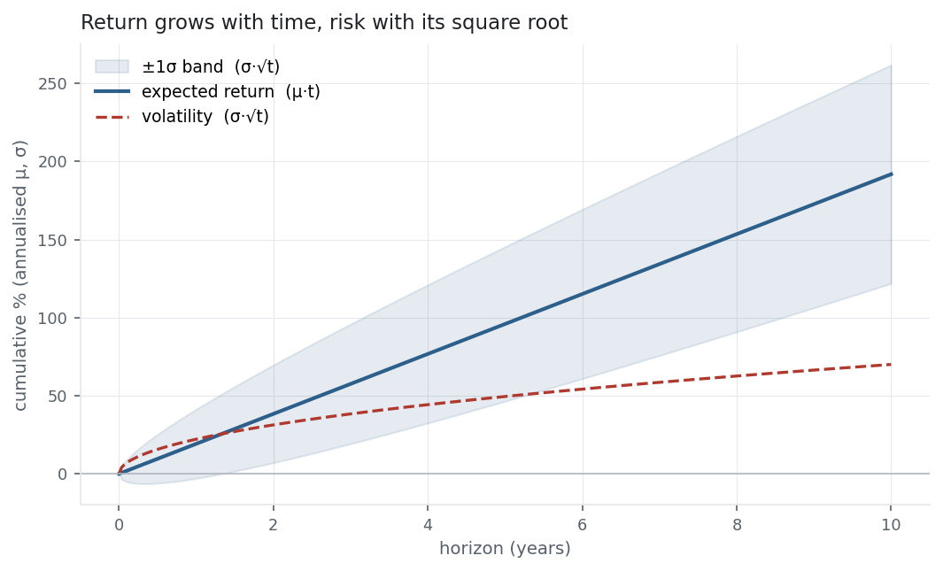
Returns and risk are measured at whatever frequency the data arrives — daily, usually — but they are quoted per year, so everything must be scaled to a common horizon. The scaling hides a subtle, important fact: return grows with time, but volatility grows with the square root of time. That one asymmetry is behind the ×252 and √252 in almost every entry so far, and it is the reason long horizons quietly favour the investor.
The equation
\mu_{\text{annual}} = N \cdot \mu_{\text{period}} \qquad \sigma_{\text{annual}} = \sqrt{N}\,\cdot \sigma_{\text{period}}
where N is the number of periods in a year (252 trading days, 52 weeks, 12 months). The mean scales linearly; the standard deviation scales with the square root — because it is variance, not σ, that adds over time:
\sigma^2_{\text{annual}} = N \cdot \sigma^2_{\text{period}}.
What each symbol means
| Symbol | Meaning |
|---|---|
| N | periods per year — 252 (daily), 52 (weekly), 12 (monthly) |
| \mu_{\text{period}},\ \mu_{\text{annual}} | the per-period and annualised mean return |
| \sigma_{\text{period}},\ \sigma_{\text{annual}} | the per-period and annualised volatility |
| \sigma^2 | variance — the quantity that adds linearly with time |
“Volatility,” in finance, almost always means the annualised standard deviation of returns.
Plain-English explanation
Say a stock earns 0.12% a day on average, with a daily standard deviation of 1.15%. To quote these per year:
- Return: multiply by 252. 0.12\% \times 252 \approx 31\%. Returns pile up linearly — twice the time, twice the expected return.
- Volatility: multiply by \sqrt{252} \approx 15.9, not 252. 1.15\% \times 15.9 \approx 18\%. Risk grows more slowly than time.
Why the difference? Because the thing that adds cleanly over time is variance, not standard deviation. Over two independent days the variances add (\sigma^2 + \sigma^2 = 2\sigma^2), so the standard deviation grows by \sqrt{2}, not 2. Extend that to a year and you get \sqrt{252}. Expected return has no such square root — it simply sums.
Why it matters in markets
This is the most-used and most-misused rule in the toolkit. Three consequences:
- The Sharpe ratio scales with √time. Numerator \times N, denominator \times\sqrt{N}, so \text{SR}_{\text{annual}} = \tfrac{N\mu}{\sqrt{N}\sigma} = \sqrt{N}\,\text{SR}_{\text{period}}. A daily Sharpe of 0.11 becomes an annual 1.7 — the same edge looks far grander annualised, which is why you must always know the frequency behind a quoted Sharpe.
- Time favours return over risk. Return grows like t, the ±σ band like \sqrt{t} (see the figure), so over long horizons the expected return pulls away from the volatility and the probability of a loss shrinks — the mathematical core of “time in the market.” The band still widens, so terminal dollar outcomes remain more dispersed even as the odds of loss fall.
- The rule assumes independence. \sigma_{\text{annual}} = \sqrt{N}\,\sigma holds only if returns are uncorrelated across time. Real returns aren’t quite: momentum (positive autocorrelation) lifts true long-horizon vol above √time, mean-reversion pulls it below. √252 is a convention, not a law.
A simple worked example
A daily mean of \mu = 0.05\% and daily volatility \sigma = 1\%:
\mu_{\text{annual}} = 0.05\% \times 252 = 12.6\%, \qquad \sigma_{\text{annual}} = 1\% \times \sqrt{252} = 15.9\%.
Watch the ratio: the daily \mu/\sigma = 0.05 becomes 12.6/15.9 = 0.79 annually — multiplied by \sqrt{252} = 15.9, not by 252. Get that one factor wrong and your annual Sharpe is off by a factor of 16.
Python implementation
import numpy as np
import pandas as pd

r = (pd.read_csv("../multi_daily.csv", index_col="Date", parse_dates=True)["NDX"]
       .pct_change().loc["2025-07-01":"2026-06-30"].dropna())

A = 252
ann_return = r.mean() * A                      # returns scale LINEARLY
ann_vol    = r.std(ddof=1) * np.sqrt(A)         # volatility scales with the SQRT
ann_sharpe = (r.mean() / r.std(ddof=1)) * np.sqrt(A)
print(round(ann_return*100, 1), round(ann_vol*100, 1), round(ann_sharpe, 2))
#   -> 30.7  18.2  1.68
The only trap is \sqrt{A} for volatility (and Sharpe) versus A for the mean. Everything else follows.
Manual / Excel calculation
| Task | Formula |
|---|---|
| Annualised return | =daily_mean * 252 |
| Annualised volatility | =daily_vol * SQRT(252) |
| Annualised Sharpe | =daily_sharpe * SQRT(252) |
Use 252 for daily data, 52 for weekly, 12 for monthly — match N to the frequency.
Financial-market example — Nasdaq 100
For NDX over the year, the daily mean of 0.12% annualises to 30.7% (×252) and the daily volatility of 1.15% to 18.2% (×√252) — the numbers behind every ratio in this library. You can watch the √time rule work by measuring volatility at different frequencies over the full history and scaling each back to a daily figure:
| Frequency | measured σ | ÷ √(periods) | implied daily σ |
|---|---|---|---|
| daily | 1.39% | — | 1.39% |
| weekly | 2.79% | ÷ √5 | 1.25% |
| monthly | 5.39% | ÷ √21 | 1.18% |
If the rule were exact, every row’s implied daily σ would match. They are close — 1.39%, 1.25%, 1.18% — but drift down as the horizon lengthens, a mild sign that NDX’s daily moves partly reverse (weekly and monthly vol come in a touch below √time). The √time rule is an excellent approximation, not a law; that small gap is exactly the autocorrelation the i.i.d. assumption ignores — which is why every desk uses √252 and every careful quant caveats it.
Same multi_daily.csv as the previous entries (yfinance, adjusted closes). Code blocks are illustrative — every figure was computed and checked against that file.
Common mistakes
- Annualising volatility with ×N. The single most common error — use ×√N. Multiplying daily vol by 252 overstates it ~16×.
- Annualising the Sharpe with the wrong factor. Sharpe scales with √N (numerator ×N, denominator ×√N); a daily Sharpe ×252 is nonsense.
- Comparing figures at different frequencies. “20% volatility” means nothing without the horizon; never compare a monthly σ to an annual one directly.
- Assuming √time is exact. It relies on i.i.d. returns; autocorrelation, fat tails, and volatility clustering all bend it. Fine as a convention, dangerous as a certainty.
- Using calendar days instead of trading days. Volatility accrues on ~252 trading days, not 365 — mixing them mis-scales everything.
- Forgetting arithmetic vs compound. ×252 annualises the arithmetic mean; the compounded figure is the CAGR, lower by the volatility drag.