Autocorrelation
How a series relates to its own past — and why returns forget but volatility remembers
Correlation measured how two different series move together. Autocorrelation asks a stranger question: how does a series move with its own past? Line a return series up against a copy of itself shifted back a day and correlate them — that lag-1 autocorrelation says whether today’s move carries any information about tomorrow’s. It is the first tool of time-series analysis, and on markets it delivers two of the most important facts in finance: prices are hard to predict, but their volatility is not.
The equation
The lag-k autocorrelation is the correlation of the series with itself k steps earlier:
\rho_k = \frac{\sum_{t=k+1}^{n}(r_t - \bar r)(r_{t-k} - \bar r)}{\sum_{t=1}^{n}(r_t - \bar r)^2}
\rho_0 = 1 always (a series is perfectly correlated with itself). The whole sequence \rho_1, \rho_2, \rho_3, \dots is the autocorrelation function (ACF).
What each symbol means
| Symbol | Meaning |
|---|---|
| \rho_k | the lag-k autocorrelation — self-correlation at a distance of k |
| r_t | the value at time t |
| r_{t-k} | the value k steps earlier |
| \bar r | the mean of the series |
| k | the lag, in periods |
| ACF | the sequence of \rho_k across lags |
\rho_k near +1 means the series trends (highs follow highs); near -1 means it mean-reverts (alternates); near 0 means the past says nothing about the present.
Plain-English explanation
Take a return series, shift a copy back by one day, and compute the ordinary correlation between the two. That is the lag-1 autocorrelation: does an up day tend to be followed by another up day (positive), a down day (negative), or neither (zero)? Repeat for a shift of 2 days, 3 days, and on, and you get the ACF — a fingerprint of the series’ memory.
To tell whether an autocorrelation is real or just sampling noise, compare it to the band \pm 1.96/\sqrt{n}. For a purely random series, 95% of the ACF should fall inside it; bars that stick out signal genuine structure. Positive autocorrelation is momentum; negative is mean reversion; a series with none is a random walk — its future is a coin flip given its past.
Why it matters in markets
Autocorrelation is where the efficient-market debate becomes measurable, and the doorway to every time-series model that follows. Two facts run through the rest of this section:
- Returns are close to unpredictable. Their ACF is small — mostly inside the band — the statistical face of the efficient market hypothesis: if you could reliably predict tomorrow’s return from the past, the edge would be arbitraged away. The faint deviations that remain are exactly where systematic strategies fish.
- Volatility is highly predictable. The ACF of squared (or absolute) returns is large and decays slowly: calm follows calm, turbulence follows turbulence. This volatility clustering is the single most important stylised fact of returns, and it is what the GARCH models later in this section exist to capture.
Autocorrelation also underlies the √time rule: that rule assumes zero autocorrelation, so the mild autocorrelation real returns carry is precisely why annualised volatility isn’t exactly √252 times the daily figure. And it is the mathematical basis of the AR models, the Hurst exponent, and the stationarity tests still to come.
A simple worked example
Two tiny series make the sign obvious. A perfectly alternating series, [+2\%, -1\%, +2\%, -1\%, +2\%, -1\%], has a lag-1 autocorrelation of -1.00: every value is followed by its opposite — perfect mean reversion. A steadily rising series, [1\%, 2\%, 3\%, 4\%, 5\%], has a lag-1 autocorrelation of +1.00: perfect trend. Real return series sit near zero, between these extremes, leaning only faintly one way or the other.
Python implementation
import numpy as np
import pandas as pd

r = (pd.read_csv("../multi_daily.csv", index_col="Date", parse_dates=True)["NDX"]
       .pct_change().dropna())

print(round(r.autocorr(lag=1), 3))          # -> -0.121   returns: small (mild mean reversion)
print(round((r**2).autocorr(lag=1), 3))     # -> 0.388    squared returns: large (clustering)

band = 1.96 / np.sqrt(len(r))               # -> ±0.036   white-noise significance band
acf  = [r.autocorr(lag=k) for k in range(1, 21)]
statsmodels.tsa.stattools.acf and plot_acf give the full function and the correlogram in one call.
Manual / Excel calculation
Lag-1 autocorrelation is just CORREL of the series against itself shifted by one row:
| Task | Formula |
|---|---|
| Lag-1 autocorrelation | =CORREL(B3:B1000, B2:B999) |
| Significance band | =1.96/SQRT(COUNT(range)) |
Shift the second range by k rows for lag k; anything smaller than the band is indistinguishable from noise.
Financial-market example — Nasdaq 100
Run the ACF on 11 years of NDX daily returns (n \approx 2{,}900, so the band is ±0.036):
| Lag | ACF of returns | ACF of squared returns |
|---|---|---|
| 1 | −0.12 | +0.39 |
| 2 | +0.04 | +0.32 |
| 5 | +0.02 | +0.21 |
| 10 | −0.04 | +0.19 |
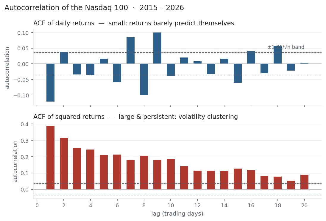
The two columns are different worlds. The returns’ autocorrelations hover around the band — the largest is the lag-1 value of −0.12, a real but small one-day mean-reversion tendency (a down day slightly favours an up day next). It is genuine: it is the same effect that gave the “buy the dip” rule a positive expectancy in Trading Metrics and pulled weekly volatility below √time in Annualisation. But it is tiny — nowhere near enough to beat costs easily, which is why markets look so close to a random walk.
The squared returns tell the opposite story: every lag out to 20 days sits far above the band, decaying only slowly from 0.39. Volatility has a long memory. You cannot forecast tomorrow’s return, but you can forecast whether tomorrow will be calm or wild — and that asymmetry is the foundation of the volatility models that close this section.
Same multi_daily.csv as the previous entries (yfinance, adjusted closes). Code blocks are illustrative — every figure was computed and checked against that file.
Common mistakes
- Running the ACF on prices, not returns. Prices are hugely autocorrelated (today’s ≈ yesterday’s) — trivially and uselessly so. Always use returns.
- Ignoring the significance band. A ρ of 0.05 looks like a signal but is noise if the band is ±0.06; small samples manufacture spurious autocorrelation.
- Reading a small return-ACF as “nothing there.” Faint but real autocorrelation (the −0.12 here) is what many systematic strategies exploit — small is not zero.
- Forgetting to check squared / absolute returns. Returns can look like white noise while their volatility clusters strongly; test both.
- Assuming autocorrelation means a tradable edge. A statistically real ρ can vanish after transaction costs — significance is not profitability.
- Using it on non-stationary data. The ACF is only meaningful for a stationary series; a drifting mean corrupts it (see the stationarity entry to come).