Cointegration

When two wandering prices stay tethered — the statistical basis of pairs trading

Cointegration: two non-stationary series whose linear combination is stationary. The hedge ratio, the Engle-Granger test, why it isn’t the same as correlation, and why genuinely cointegrated pairs are rare.

Correlation asks whether two assets move together day to day. Cointegration asks something deeper and rarer: whether two prices, each free to wander wherever it likes, are nonetheless tied by an invisible leash — so that some combination of them never strays far from a fixed level. That combination, the spread, is stationary and mean-reverting, which makes it tradable. Cointegration is the honest statistical foundation of pairs trading — and, as the data will show, far rarer than the correlations mistaken for it.

The equation

Two series X_t and Y_t are cointegrated if each is non-stationary (integrated of order 1) but a linear combination is stationary:

X_t \sim I(1), \quad Y_t \sim I(1), \quad \text{but} \quad s_t = Y_t - \beta X_t \sim I(0).

\beta is the hedge ratio and s_t is the spread. The Engle-Granger test finds \beta by OLS, then runs an ADF test on the residual spread — if the spread is stationary, the pair is cointegrated.

What each symbol means

Symbol	Meaning
X_t,\ Y_t	the two price series (both non-stationary)
I(1)	“integrated of order 1” — non-stationary, but its difference is stationary
I(0)	stationary
\beta	the hedge ratio — units of X to short against one Y
s_t	the spread, Y_t - \beta X_t — stationary when the pair is cointegrated

Correlation acts on returns; cointegration acts on price levels. A pair can be one without the other.

Plain-English explanation

Picture two drunks leaving a bar, each staggering at random — neither has any idea where they’re going (two random walks, both non-stationary). Now tie them together with a short rope. Individually they still wander anywhere, but the distance between them can never grow large: it snaps back. That distance is the spread, and its refusal to wander is cointegration.

For prices, cointegration says two assets share a long-run equilibrium. Each price is a random walk on its own, but a specific weighted difference — the spread — is stationary, oscillating around a fixed mean and reverting to it. Find such a pair and you have something to trade: when the spread stretches unusually wide (say +2σ), you bet on it snapping back — short the expensive leg, long the cheap one — and close when it returns to the mean. That is pairs trading, and cointegration is what makes it more than wishful thinking.

Why it matters in markets

Cointegration is the difference between a real pairs trade and a data-mined mirage, and its central lesson is that correlation is not cointegration. Correlation measures whether returns move together in the short run; cointegration measures whether prices stay tied in the long run. Two stocks can be highly correlated yet drift apart forever (correlated, not cointegrated), or barely correlated day-to-day yet anchored to the same level (cointegrated, not correlated). Trading a pair because it’s correlated, without checking cointegration, is how “market-neutral” books blow up when the spread that “always reverted” simply keeps widening.

The catch is that genuine cointegration is rare and fragile: it needs a real economic link (the same commodity, a merger, two share classes, a dual listing), it must survive out-of-sample, and it can break the moment the relationship that caused it changes. The Engle-Granger recipe — regress for \beta, ADF-test the spread — is the minimum honest check, and even a passing test can be a fluke without an economic story.

A simple worked example

Take a shared random-walk trend W_t and build two prices on it: X_t = 100 + W_t + \text{noise} and Y_t = 50 + 2W_t + \text{noise}. Each is non-stationary — an ADF test can’t reject a unit root in either. But because Y \approx 2X, the combination Y_t - 2X_t cancels the shared trend and leaves only noise: a stationary spread. Regressing Y on X recovers the hedge ratio \beta = 1.99 (essentially the true 2), and an ADF test on the spread gives p < 0.001 — decisively stationary. That is a textbook cointegrated pair, and its spread (the figure) is what you would trade.

Python implementation

from statsmodels.tsa.stattools import coint, adfuller
import numpy as np

# X, Y are two price (level) series
pval   = coint(X, Y)[1]                    # Engle-Granger: p < 0.05 => cointegrated
beta   = np.polyfit(X, Y, 1)[0]            # hedge ratio (OLS slope of Y on X)
spread = Y - beta * X
print(round(pval, 4), round(adfuller(spread)[1], 4))   # coint p, spread ADF p

z = (spread - spread.mean()) / spread.std()            # trade |z| > 2, exit near 0

coint runs the whole Engle-Granger procedure; the manual polyfit + adfuller on the residual is the same thing, and shows exactly what the test does.

Manual / Excel calculation

There is no spreadsheet shortcut — cointegration needs a regression plus an ADF test, so use statsmodels.coint (Python) or R’s urca / egcm. The two-step logic you can follow anywhere: (1) regress Y on X to get \beta and the residual spread; (2) test whether that spread is stationary. A stationary spread means the pair is cointegrated.

Financial-market example — Nasdaq 100

Here honesty beats a tidy story. Testing every pair in the basket over 2015–2026 — highly correlated names included — not one is cointegrated:

Pair	return correlation	cointegration p
NDX ~ MSFT	+0.81	1.00
NDX ~ AAPL	+0.78	0.19
AAPL ~ MSFT	+0.64	0.98
MSFT ~ NVDA	+0.59	0.98

Every p-value is far above 0.05: no stationary spread exists. NDX and MSFT rise together with a 0.81 return correlation, yet their price levels drift apart over the decade — correlated, not cointegrated. This is the rule, not the exception: most stock pairs share no long-run tether, which is exactly why real pairs trading hunts narrow, economically linked relationships (a company and its tracking stock, two share classes, a commodity and its producer) rather than “these two charts look similar.”

A constructed cointegrated pair: both prices (top) wander freely and non-stationarily, but their spread Y − 1.99·X (bottom) oscillates around a constant mean between ±2σ bands — stationary and mean-reverting, the tradable object.

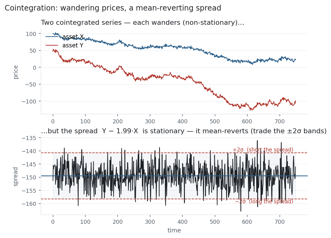
The figure shows what the exception looks like — a constructed cointegrated pair. Both prices wander freely, but their spread Y - 1.99X oscillates around a constant mean and snaps back every time it stretches: stationary, mean-reverting, tradable. That mean-reverting spread is the whole prize of cointegration — and finding a genuine one in live markets is the hard part.

Basket pairs from multi_daily.csv (yfinance); cointegration via statsmodels (Engle- Granger). The spread figure is a constructed cointegrated pair, since no basket pair qualifies — which is itself the point.

Common mistakes

• Confusing correlation with cointegration. Correlation is short-run co-movement of returns; cointegration is a long-run tether in prices. High correlation does not imply a stationary spread.
• Trading a pair without testing the spread. “It always reverts” is a chart illusion until an ADF test on the spread rejects a unit root — and even then, out-of-sample.
• Data-mining pairs. Test enough pairs and some pass by chance; without an economic reason, a passing cointegration test is likely spurious.
• Assuming cointegration is permanent. Relationships break (mergers, business shifts); a spread that reverted for years can suddenly trend — how pairs books blow up.
• Ignoring the hedge ratio. The spread is Y - \beta X, not simply Y - X; the wrong \beta leaves a non-stationary, untradable spread.
• Running it on returns. Cointegration lives in the non-stationary price levels; test it on stationary returns and you’re testing the wrong thing.