Cross-Entropy Loss
Scoring probabilities by their surprise — the loss that pairs with sigmoid and softmax
The sigmoid and softmax entries produced probabilities; cross-entropy is how you grade them. It is the classification counterpart of mean squared error — the default loss whenever a model outputs a probability rather than a number — and it works by measuring surprise: how unlikely the true answer looked under the model’s prediction. Confident and right costs almost nothing; confident and wrong costs a fortune. That asymmetry, plus a gradient that combines with sigmoid and softmax into something remarkably clean, is why cross-entropy sits at the end of essentially every classifier.
The equation
For a binary label y \in \{0,1\} and predicted probability p:
L = -\big[\,y\log p + (1-y)\log(1-p)\,\big]
For K classes with a one-hot label y and predicted distribution p (from softmax):
L = -\sum_{k=1}^{K} y_k \log p_k = -\log p_{\text{true}}
Only the probability assigned to the correct class matters; the loss is its negative log.
What each symbol means
| Symbol | Meaning |
|---|---|
| L | the cross-entropy loss |
| y | the true label (0/1, or a one-hot vector) |
| p | the predicted probability (or distribution) |
| p_{\text{true}} | probability the model gave to the correct class |
| \log | natural log (nats) or \log_2 (bits) |
| K | the number of classes |
Plain-English explanation
Cross-entropy scores a probabilistic prediction by how surprised it was by the truth. If the true class was the one your model called 90% likely, the surprise -\log(0.9) = 0.11 is small; if the truth was a class you gave only 10%, the surprise -\log(0.10) = 2.3 is large; if you gave it 1%, -\log(0.01) = 4.6 — the penalty climbs without bound as your probability for the right answer approaches zero. That is the defining behaviour: cross-entropy is gentle when you’re right and merciless when you were confidently wrong. A hedged 50/50 guess always costs \log 2 \approx 0.69, the price of admitting you don’t know.
For binary problems the formula has two terms but only one ever fires: if the label is 1 you pay -\log(p), if it’s 0 you pay -\log(1-p). For many classes it collapses to -\log(p_{\text{true}}) — the model is graded solely on the probability it assigned to what actually happened. Two facts make this the “right” loss. Minimising it is exactly maximum-likelihood estimation (you are maximising the probability the model assigns to the observed data), and its gradient, when the probabilities come from a sigmoid or softmax, simplifies to just (p - y): predicted minus actual. That clean signal — no vanishing gradient even when the model is confidently wrong — is why softmax-plus-cross- entropy is the universal final layer, and why pairing sigmoid with squared error instead is a mistake.
Why it matters in markets
Cross-entropy is a proper scoring rule: it can’t be gamed, because the only way to lower your expected loss is to report probabilities that are actually calibrated. That makes it the honest scorekeeper for any probabilistic market forecast — and on near-efficient markets, honesty means humility. Because the loss explodes for confident-wrong predictions, a model that declares a bold “80% up” and is wrong is punished far more than one that admits “56% up”; over many days, the calibrated, near-base-rate forecaster wins. This is the mathematical reason not to bet the farm on a thin edge: the scoring rule itself rewards probabilities that match reality.
It is also the cleanest measure of how much a model actually knows. The cross-entropy of always predicting the base rate equals the entropy of the labels (the next entry) — the irreducible surprise in the data — and any model can only score below that by the amount of real information it captures. The gap between a model’s cross-entropy and the base-rate cross-entropy is the information it adds. On the Nasdaq, as the figure shows, that gap is almost nothing.
A simple worked example
The true label is y = 1 and the model predicts p = 0.8. The loss is -\log(0.8) = 0.22 — a modest penalty for a mostly-right call. Now suppose the model was confidently wrong, predicting p = 0.2 for a label that turned out to be 1: the loss jumps to -\log(0.2) = 1.61, over seven times worse. Compare what squared error charges for the same mistake: (1 - 0.2)^2 = 0.64, less than half. Cross-entropy’s steeper penalty for confident errors is exactly what makes it train classifiers faster and keeps them honest.
Python implementation
import numpy as np

def binary_cross_entropy(y, p, eps=1e-12):
    p = np.clip(p, eps, 1 - eps)                  # avoid log(0)
    return -np.mean(y*np.log(p) + (1-y)*np.log(1-p))

# categorical: -mean(log of the probability given to the true class)
# (sklearn.metrics.log_loss handles both binary and multi-class)
The clip matters: a prediction of exactly 0 or 1 gives an infinite loss, so probabilities are nudged off the boundary. The gradient of cross-entropy through a sigmoid/softmax is simply p - y.
Manual / Excel calculation
For a binary prediction, cross-entropy is one formula — =-(y*LN(p) + (1-y)*LN(1-p)) — averaged down the column. For multi-class it is just =-LN(prob_of_true_class) per row. Use LN for nats or LOG(x, 2) for bits.
Financial-market example — Nasdaq 100
Grade three forecasters of “will the Nasdaq rise tomorrow?” by their cross-entropy (log loss) over eleven years. A coin flip that always says 0.50 scores \log 2 = 0.6931. A constant that always predicts the base rate, 0.56, scores 0.6859 — and that number is exactly the entropy of the up/down labels, the irreducible uncertainty. The logistic model fitted on today’s return scores 0.6854.
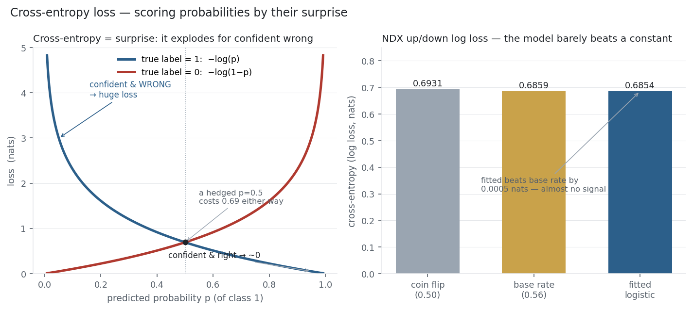
Read the gaps. The fitted model beats the base-rate constant by 0.0005 nats — a rounding error. The base rate itself beats the coin flip by 0.007, just from knowing the market drifts up 56% of the time. In other words, essentially all of the (tiny) edge is in the unconditional base rate, and almost none in the conditioning on today’s return. Cross-entropy makes the efficient-market verdict quantitative and unforgiving: a model that genuinely predicted direction would post a visibly lower log loss, and this one doesn’t. The left panel is why to trust that verdict — the loss would have savaged an over-confident model, so these near-base-rate scores are the honest ones.
Same multi_daily.csv as the previous entries (yfinance, adjusted closes). Log loss via sklearn.metrics.log_loss (natural log / nats); the base-rate score equals the labels’ entropy by construction. Every number was checked.
Common mistakes
- Feeding it un-normalised scores. Cross-entropy expects probabilities; apply sigmoid/softmax first (or use a “from logits” version that fuses the two for numerical stability).
- Taking the log of zero. A predicted 0 or 1 for the wrong class is infinite loss; clip probabilities away from the boundary.
- Using squared error for classification. MSE + sigmoid is non-convex and learns slowly; cross-entropy gives the clean (p-y) gradient.
- Confusing nats and bits. Natural log gives nats, \log_2 gives bits; don’t compare across bases (0.69 nats = 1.0 bit at p=0.5).
- Reading log loss as accuracy. It grades calibrated probabilities, not just the top-1 label; a well-calibrated hedger can beat an over-confident guesser on log loss while tying on accuracy.
- Forgetting the base-rate baseline. A log loss only means something against the label entropy; beating a constant base-rate predictor is the real bar — and, on markets, a high one.