Kelly Criterion
The bet size that maximises long-run growth — and why you should bet less than it says
Every other entry measures a strategy; Kelly acts on one. Given an edge, how much of your capital should you bet? Too little and you leave growth on the table; too much and you go broke even with a winning system. The Kelly criterion is the exact answer — the bet fraction that maximises the long-run compound growth rate of wealth. It is the bridge from “how good is the edge” to “how much to bet,” and it wires straight back to the Sharpe ratio.
The equation
For a bet paying net odds b with win probability p (and loss probability q = 1-p), the Kelly fraction is:
f^* = \frac{bp - q}{b} = \frac{p(b+1) - 1}{b}
For a continuous investment with expected excess return \mu and variance \sigma^2, it becomes a leverage:
f^* = \frac{\mu}{\sigma^2}
Both maximise the expected logarithm of wealth — equivalently, the compound growth rate.
What each symbol means
| Symbol | Meaning |
|---|---|
| f^* | the optimal fraction of capital to bet (a leverage if >1) |
| p,\ q | win and loss probabilities (q = 1-p) |
| b | net odds — the amount won per unit staked on a win |
| bp - q | the edge — expected profit per unit staked |
| \mu | expected excess return, over the risk-free rate |
| \sigma^2 | the variance of returns |
The discrete form is edge over odds; the continuous form is excess return over variance. Both say the same thing: bet more when the edge is bigger, less when the risk is bigger.
Plain-English explanation
You have a coin that lands heads 60% of the time and pays even money — a real edge. But how much of your bankroll do you stake each flip? Bet everything and one tail ruins you; bet nothing and you never grow. Kelly finds the sweet spot that grows your money fastest over many flips: here f^* = p - q = 0.6 - 0.4 = 0.2, so stake 20% each time.
The crucial idea is that Kelly maximises growth, not expected profit. Maximising expected profit would tell you to bet everything (it has the highest average) — but that “average” is propped up by rare enormous outcomes while the typical path goes to zero. Kelly instead maximises expected log-wealth, which is exactly the compound growth rate that determines where your money actually ends up.
Why it matters in markets
The library up to here has been diagnosis — return, risk, Sharpe, drawdown. Kelly is the prescription: it turns an edge into a position size. But its real lessons are about restraint.
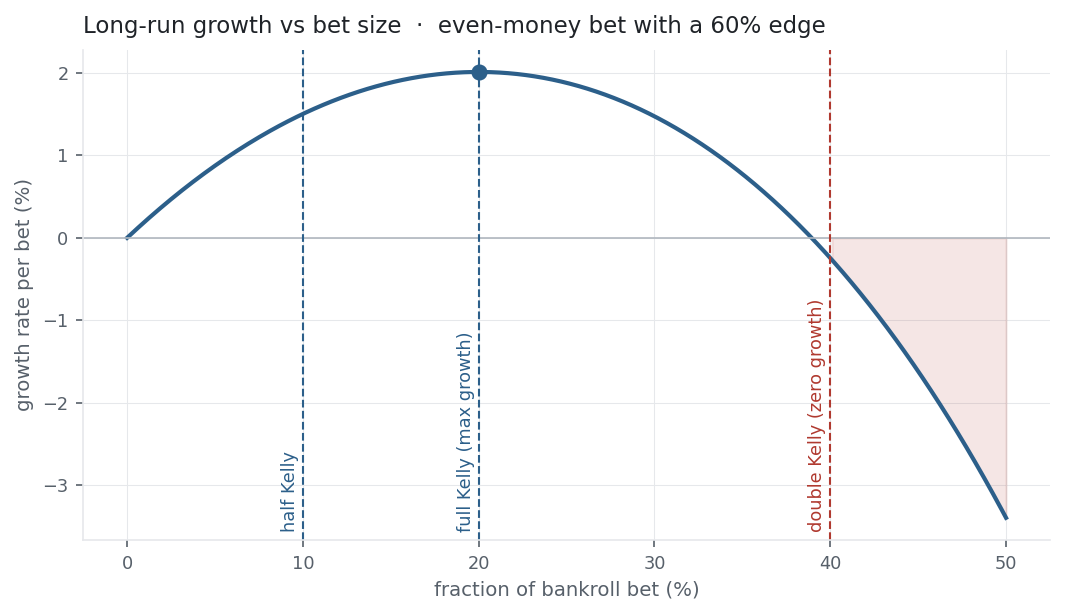
The growth-versus-bet-size curve (below) is a hump: growth climbs to a peak at full Kelly, then falls, and crosses zero at exactly twice Kelly. So over-betting is punished twice over — past the peak you take more risk for less growth, and past 2f^* a positive-edge strategy loses money in the long run. Betting beyond Kelly isn’t bold, it’s mathematically self-destructive.
That is why practitioners bet fractional Kelly, usually half. Half-Kelly captures about 75% of the growth for roughly a quarter of the variance, and it buys a margin of safety against the deeper problem: Kelly assumes you know p, b, \mu, and \sigma exactly, and you never do. Overestimate your edge and full Kelly silently puts you past the peak.
And the connection that ties the whole library together: for a continuous asset f^* = \text{SR}/\sigma, and the maximum achievable growth rate is r_f + \tfrac{1}{2}\text{SR}^2 — half the Sharpe ratio squared. Kelly is where the Sharpe ratio stops describing performance and starts dictating leverage.
A simple worked example
The 60%-heads, even-money coin: p = 0.6, q = 0.4, b = 1.
f^* = \frac{bp - q}{b} = \frac{(1)(0.6) - 0.4}{1} = 0.2 \quad\Rightarrow\quad \text{stake } 20\%.
At full Kelly the long-run growth is about 2.01% per flip; at half-Kelly (10%) it is 1.50% — still 75% of the growth, with far smaller swings. Stake double Kelly (40%) and growth turns slightly negative: a winning coin that loses money, purely from over-betting.
Python implementation
import numpy as np
import pandas as pd

# discrete Kelly: win prob p, net odds b
p, b = 0.60, 1.0
f_star = (b*p - (1 - p)) / b
print(round(f_star, 2))                          # -> 0.2   (stake 20% of bankroll)

# continuous Kelly on NDX (full history)
r = (pd.read_csv("../multi_daily.csv", index_col="Date", parse_dates=True)["NDX"]
       .pct_change().dropna())
A, rf = 252, 0.04
mu  = r.mean() * A - rf                           # annualised excess return
var = (r.std(ddof=1) * np.sqrt(A)) ** 2           # annualised variance
f   = mu / var                                   # Kelly leverage
sharpe = mu / var**0.5
print(round(f, 2), round(sharpe, 2))             # -> 3.1  0.69
print(round(rf + 0.5*sharpe**2, 3))              # -> 0.275   max growth = rf + 0.5*SR^2
f > 1 means Kelly wants leverage. In practice you halve it — and never trust a single-sample estimate of \mu.
Manual / Excel calculation
Kelly is a single division; the hard part is honest inputs.
| Task | Formula |
|---|---|
| Discrete Kelly | =(b*p - (1-p)) / b |
| Continuous Kelly | =excess_return / variance |
| Half Kelly | =0.5 * (the above) |
Financial-market example — Nasdaq 100
Treat NDX as one asset. Over its full 2015–2026 history its annualised excess return (over 4%) was 15.2% and its volatility 22.1%, so:
f^* = \frac{\mu}{\sigma^2} = \frac{0.152}{0.221^2} = 3.1.
Full Kelly says borrow to hold 3.1× NDX, and the growth that buys is r_f + \tfrac{1}{2}\text{SR}^2 = 4\% + \tfrac{1}{2}(0.69)^2 = 27.5\% a year. Two warnings are baked into those numbers. First, 3.1× leverage through the 35.6% drawdown of 2022 would have meant a >100% loss — ruin; the theoretical optimum ignores that you have to survive the path. Second, the estimate sensitivity is savage: run the same formula on just the recent high-Sharpe year and it demands 8× leverage. The edge you feed in is never as certain as Kelly assumes — which is the entire case for betting a fraction of it.
Same multi_daily.csv as the previous entries (yfinance, adjusted closes). Code blocks are illustrative — every figure was computed and checked against that file.
Common mistakes
- Betting full Kelly. It maximises growth in theory, but with brutal drawdowns and no margin for estimation error. Half-Kelly is the practical default.
- Over-betting past 2f^*. Beyond twice Kelly a positive-edge strategy has negative long-run growth — more aggression, less money.
- Trusting the inputs. Kelly assumes p, b, \mu, \sigma are known exactly; overestimating the edge silently pushes you past the peak. Garbage in, ruin out.
- Confusing it with maximising expected return. Max expected return says bet everything; Kelly maximises growth (expected log-wealth), which is what compounds.
- Applying it per-trade in isolation. Correlated bets, fat tails, and the risk of total loss all break the clean formula — real sizing sits well below the naive number.
- Ignoring your drawdown tolerance. The right fraction is also the one you can actually survive; an optimal bet you abandon at the bottom was never optimal for you.