Backpropagation as an Algorithm
Reverse-mode automatic differentiation — the whole gradient in one backward pass, exact and cheap
The neural network learns by gradient descent, which needs the gradient of the loss with respect to every weight — and in a network with thousands or millions of them, computing that gradient is the entire problem. Backpropagation is the answer, and it is worth separating the two things it is. As mathematics it is just the chain rule applied backward through the network — that derivation, with the \delta error-signal equations and a worked numeric pass, lives in the Equation Library entry. As an algorithm — the subject of this page — it is reverse-mode automatic differentiation: the reason you can get the gradient of one scalar loss with respect to a million parameters in a single backward pass, exactly, at essentially the cost of one forward pass. That efficiency is not a detail. It is the reason deep learning exists at all.
1. What problem does it solve?
Computing \nabla_\theta L — the gradient of a scalar loss with respect to every parameter \theta in the model — efficiently and exactly. It is not itself a model or a learner; it is the subroutine every neural network’s training loop calls to find out which way is downhill. The naive alternative, nudging each weight and measuring the change in loss (finite differences), costs a full forward pass per parameter and is hopeless at scale. Backpropagation gets the complete gradient in one backward pass. Everything modern — from a small market net to a large language model — depends on this one algorithm.
2. What assumptions does it make?
That the model and loss form a differentiable computational graph: a composition of operations each of which has a known local derivative (a Jacobian). It assumes a single scalar output (the loss) — which is exactly why reverse-mode is the right choice: with one output and many inputs, one backward sweep yields all the input gradients at once. And it assumes you can store the forward pass’s intermediate values, because the backward pass reuses them. Where a piece of the graph is non-differentiable (a hard threshold, a discrete sample), you need a surrogate gradient or a reparameterisation.
3. What does it operate on?
Not data directly, but the computation graph the forward pass builds. Its defining resource cost is therefore memory: to compute each layer’s gradient on the way back, backprop needs that layer’s activations from the way forward, so it caches them all. That activation memory — proportional to the network’s width times depth times batch size — is the real bottleneck for large models, and the reason techniques like gradient checkpointing (recompute activations instead of storing them) exist, trading compute for memory. Compute, by contrast, it barely touches: the backward pass costs about what the forward pass does.
4. How does it work?
Two passes over the graph. The forward pass evaluates the network, caching each operation’s inputs and outputs, and ends at the scalar loss. The backward pass starts with \partial L/\partial L = 1 and walks the graph in reverse; at each operation it multiplies the incoming gradient by that operation’s local Jacobian — a vector-Jacobian product — and passes the result to the operation’s inputs, accumulating \partial L/\partial \theta at every parameter along the way. For a layered network this reverse sweep is the \delta recurrence derived in the Equation Library; automatic-differentiation frameworks simply run the same idea over an arbitrary graph, which is what loss.backward() does.
Why reverse mode? Because differentiation can sweep either direction, and the costs are asymmetric. Forward mode propagates derivatives input-to-output and needs one sweep per input — fine for many outputs and few inputs. Reverse mode propagates output-to-input and needs one sweep per output — and a loss has exactly one output, so a single sweep delivers all P parameter gradients. That is the whole efficiency argument, and it is dramatic in practice.
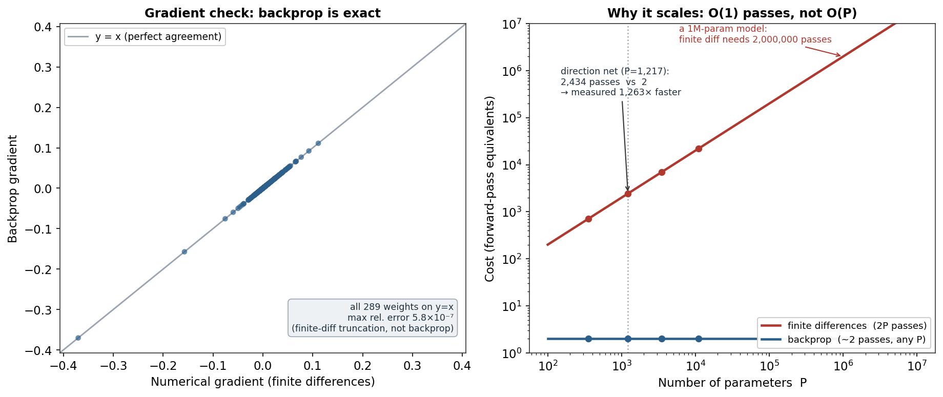
Two facts anchor the figure. First, backprop is exact: checked against central finite differences on every weight of a small net, the two agree to a relative error of 5.8\times10^{-7} — and that residual is the finite differences’ own truncation error, not backprop’s, which is exact to machine precision. (This “gradient check” is the standard way to validate a hand-written backward pass.) Second, it is cheap in a way that scales: the backward pass is a constant ~2 forward-pass equivalents regardless of P, while finite differences cost 2P. Measured on real networks the speedup was 397× at 353 parameters, 1,263× at 1,217, and 6,564× at 11,000 — the gap widening without limit. A million-parameter model would need two million forward passes to differentiate numerically; backprop still needs two.
5. What are its strengths?
- Exact. It computes the true gradient to machine precision, unlike the approximate, noise-prone finite-difference estimate.
- O(1) passes for the whole gradient. One backward pass yields every parameter’s gradient, independent of how many there are — the reason training large models is feasible.
- General (automatic differentiation). The same reverse sweep differentiates any differentiable graph, not just layered nets — the engine inside PyTorch, TensorFlow, and JAX.
- Automatic.
loss.backward()builds and differentiates the graph for you; you never hand-derive gradients. - Composable. It just supplies gradients, so it pairs with any optimiser (SGD, Adam) and any differentiable loss or regulariser.
6. What are its weaknesses?
- Memory-hungry. Caching every activation for the backward pass is the dominant cost at scale (mitigated by gradient checkpointing).
- Needs differentiability. Hard thresholds and discrete sampling break it without surrogate gradients or reparameterisation.
- Sequential. The backward pass depends on the completed forward pass and unwinds layer by layer, limiting parallelism across depth.
- Inherits vanishing/exploding gradients. It faithfully propagates whatever the graph dictates — including the saturating-activation collapse — so it exposes, but doesn’t fix, those pathologies.
- Not a learner by itself. It only computes gradients; it needs an optimiser and a loss to actually train anything.
7. How could it apply to markets?
Backprop is the engine, not the edge. It optimises flawlessly — which is precisely why a falling training loss proves nothing about a market model. The Equation Library’s Nasdaq experiment makes the point: backprop drives a net’s training loss steadily down while its validation loss climbs and out-of-sample accuracy lands at 50%, below the base rate. The algorithm worked perfectly; all it found was noise. What backprop genuinely buys a quant is feasibility — reverse-mode differentiation is what lets you train a model with thousands or millions of parameters on market data at all. The right-hand figure is the practical stakes: at the direction net’s 1,217 parameters backprop is already 1,263× faster than differentiating numerically, and beyond a few thousand parameters finite differences simply stop being an option. The honest verdict on next-day direction is unchanged; backpropagation is what makes reaching that verdict — and training every model that can — computationally possible.
8. What does the Python code look like?
# The backward pass for one layer, then the gradient check that validates it.
def backward(cache, y):
    # cache holds forward-pass activations; returns dL/dW for every layer
    ...                                  # the delta recurrence (see Equation Library)

# GRADIENT CHECK — the standard way to trust a hand-written backward pass:
import numpy as np
g_backprop = flatten(backward(cache, y))
g_numeric  = np.array([                                  # central finite differences
    (loss(theta + e*unit(i)) - loss(theta - e*unit(i))) / (2*e) for i in range(P)])
rel_err = np.abs(g_backprop - g_numeric).max() / (np.abs(g_backprop).max() + 1e-12)
assert rel_err < 1e-5                                    # ours: 5.8e-7

# In practice you never write backward() — autodiff does it:
loss = loss_fn(model(X), y)
loss.backward()          # reverse-mode autodiff fills every parameter's .grad
optimizer.step()         # gradient descent uses those grads (a separate step)
The gradient check is worth knowing: whenever you implement a custom gradient, verify it against finite differences on a tiny input before trusting it. In production, loss.backward() is backprop — reverse-mode autodiff over the graph your forward pass built.
9. How would I explain it to a supervisor?
“Backpropagation is reverse-mode automatic differentiation: a forward pass evaluates the network and caches intermediates, then a backward pass applies the chain rule from the loss inward, multiplying by each operation’s local Jacobian to accumulate the gradient for every parameter. The key property is that because the loss is a single scalar, one backward pass produces all the parameter gradients — so it costs about two forward passes regardless of whether the model has a hundred parameters or a billion, whereas finite differences cost two per parameter. I verified both: it matches numerical gradients to about 1e-7 — that gap is the finite-difference error, not backprop’s — and it was over a thousand times faster at just 1,200 parameters. It’s the algorithm that makes training any neural network feasible; it computes the gradients, and an optimiser like Adam then uses them.”
The chain-rule derivation and \delta equations are in the Equation Library; this page is the algorithm/efficiency view. Gradient check: a 289-parameter ReLU network, backprop versus central finite differences (max relative error 5.8\times10^{-7}). Efficiency: forward-pass counts are exact (2 vs 2P); wall-clock speedups (397×–6,564×) were measured on networks from 353 to 11,009 parameters. Every number was checked.